1. Introduction
CivilTerrain 3D creates and edits digital terrain models (TIN) and computes earthworks. It is intended for land surveyors, civil engineers, construction companies, earthwork and road contractors, and LiDAR/drone survey professionals.
With CivilTerrain 3D you can:
- import points from CSV/TXT/XYZ, DXF, LAS/LAZ, PLY/OBJ, LandXML and DEMs (GeoTIFF, ASCII Grid, SRTM, BIL / FLT);
- build a triangulated terrain model with breaklines, boundaries and holes;
- generate labelled and smoothed contours;
- compute cut/fill volumes between surfaces or against an elevation;
- design excavations whose slopes intersect the real ground;
- produce longitudinal profiles and cross sections, and re-create them at the same positions for re-measurement;
- export drawings and reports to DXF, PDF, Excel, LandXML, GeoTIFF and more.
.prj or the tile name, and a transformation into the project's system (e.g. WGS 84 → GGRS87); only the project area of large DEMs and keeping every n-th cell; TIFFs without georeference through their world file (.tfw); surface export as an ESRI ASCII Grid.System requirements
| Operating system | Windows 10 (1809 or later) or Windows 11, 64-bit |
|---|---|
| Memory | 4 GB (8 GB+ recommended for point clouds) |
| Graphics | Graphics card with OpenGL support (all modern cards) |
| Disk | ~150 MB for the installation |
| Internet | Only for license activation/validation and updates |
2. Installation and licensing
2.1 Installation
- Download
CivilTerrain3D-Setup-x.y.z.exefrom www.civilshop.gr/demos.aspx. - Run it. If Windows SmartScreen appears, click More info → Run anyway.
- Accept the license terms, choose a folder and optionally a desktop icon and the association of
.ct3dproject files. - The program starts at the end. The Start menu also contains a shortcut to the sample data.
No other software is required. Uninstall from Windows Settings → Apps.
2.2 Free 14-day trial
From the first start you have 14 days of full functionality without a key. The remaining days are shown in the window title and in the status bar (bottom right). After the trial the program runs in viewer mode: you can open and view projects, but saving, exports, reports, excavation and sections are disabled until a license is activated. Your projects are kept.
2.3 License activation
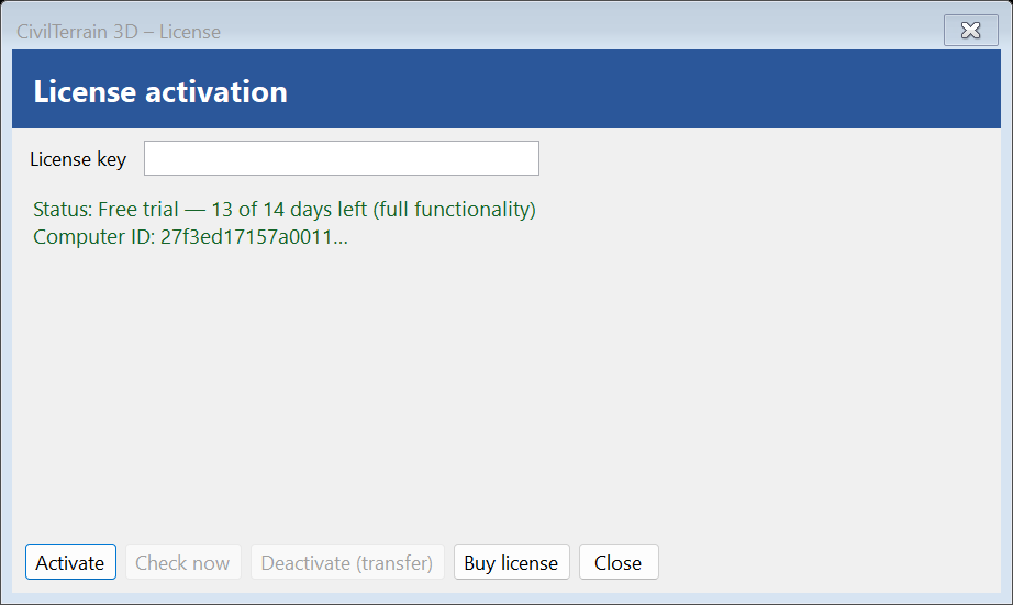
- Open File → License… or click the license indicator in the status bar.
- Type or paste your license key (e.g.
CIVILTERRA-XXXXX-…). - Click Activate. An Internet connection is required.
| Button | Function |
|---|---|
| Activate | Binds the license to this computer. |
| Check now | Checks the license status on the server immediately. |
| Deactivate (transfer) | Releases the license from this computer so it can be activated on another one. |
| Buy license | Opens the shop in your browser. |
Possible messages: license expired, revoked, suspended, all activations are used by other computers (deactivate one first), key does not exist. If your license contains specific modules, the other functions show a notice.
2.4 Updates
At every start and from File → Check for updates the program looks for a newer version. Updates are provided while the license's update subscription is active; after it expires, the installed version keeps working.
3. The user interface
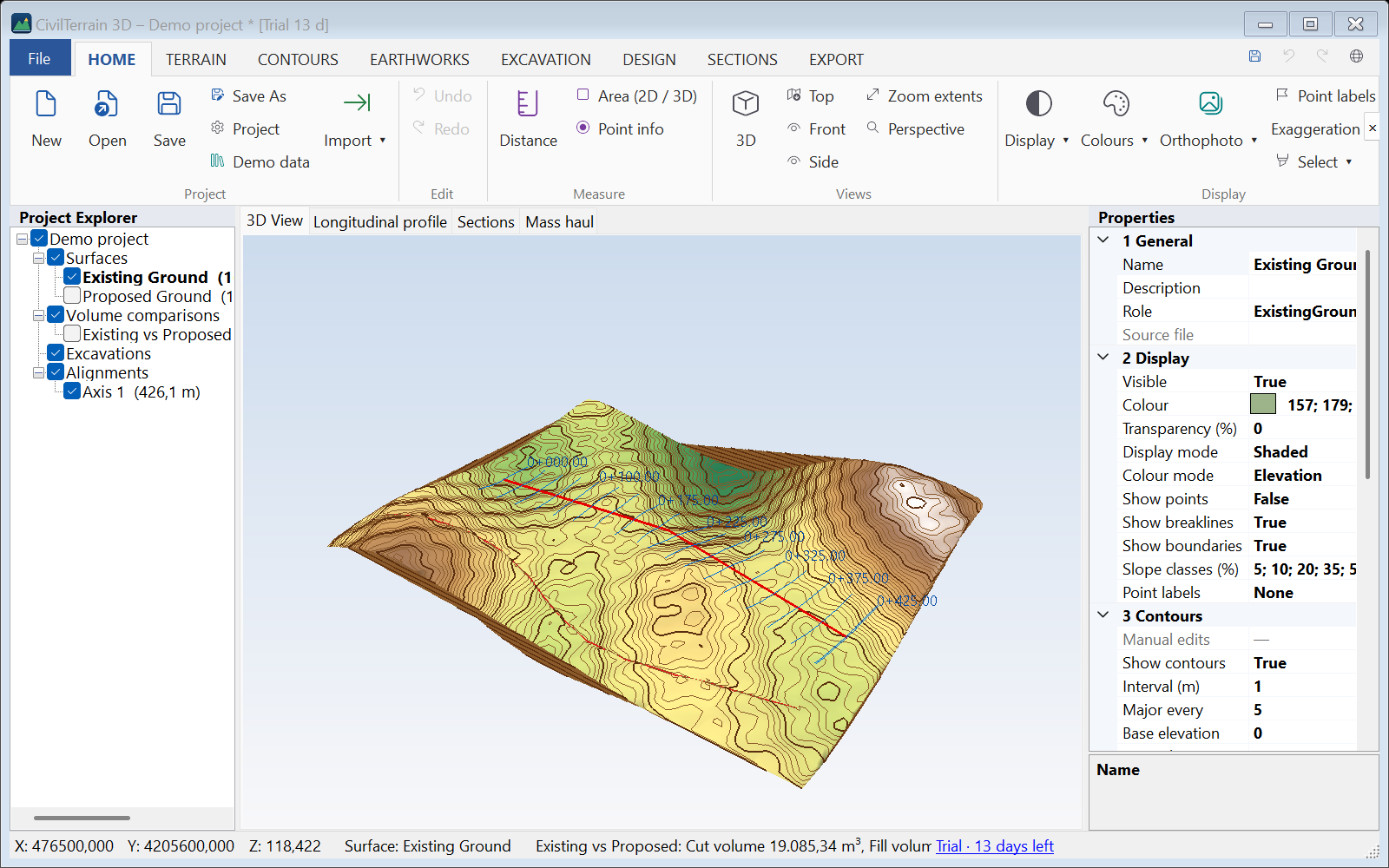
| Area | Description |
|---|---|
| Ribbon | Commands organised in tabs: HOME, TERRAIN, CONTOURS, EARTHWORKS, EXCAVATION, DESIGN, SECTIONS, WATER, EXPORT. Double-click a tab to collapse/expand the ribbon. |
| File (blue button) | New, Open, Save, Save As, Project settings, Recent projects, License, Check for updates, Classic toolbars, Theme (section 3.3), About, Exit. |
| Quick access (top right) | Save, Undo, Redo, switch language Ελληνικά/English. |
| Project Explorer | Tree of every object of the project (section 3.2). The check box shows/hides. Click selects (the selected surface becomes the active one, in bold). Double-click zooms to it. Right-click opens a menu (Rebuild, Duplicate, Statistics, Delete…). |
| Centre | Tabs 3D View, Longitudinal profile, Sections, Mass haul (mass-haul diagram, section 17.5). |
| Properties | Settings of the selected item (display, contours, TIN, statistics, volume results…). Changes apply immediately. |
| Status bar | X, Y, Z under the cursor, active surface, messages/tool prompts, progress, license status and coordinate system. |
3.1 Ribbon tabs











In a narrow window (e.g. a laptop), when the groups of a tab do not fit, the ribbon scrolls: with the ‹ › arrows at its ends or with the mouse wheel over it. If the tabs do not fit beside the quick-access buttons, they get narrower.
3.2 Project Explorer
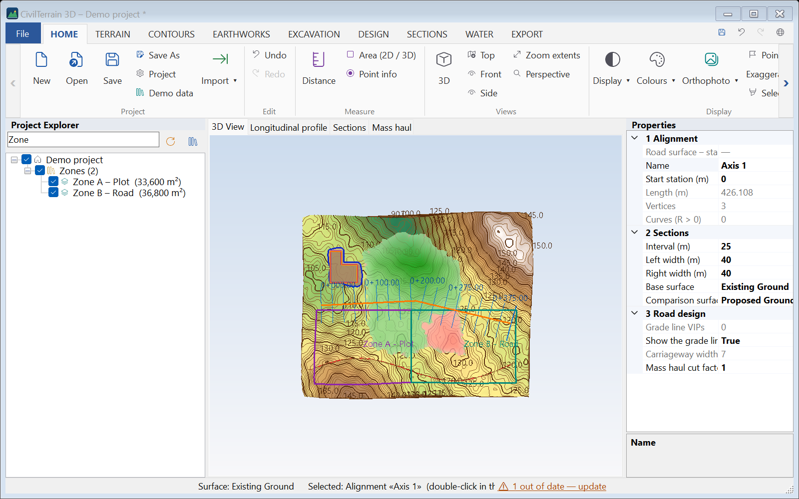
The Project Explorer tree shows every object of the project with icons and a count per collection. Above the tree are a Search box and two buttons: Update all and Item list. When the tree is rebuilt, it keeps which nodes are open and which one is selected.
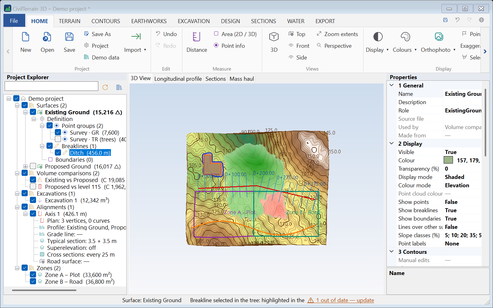
The definition of every surface
Below every surface, the Definition node shows what takes part in its TIN (and the maximum triangle edge, if set):
- Point groups – the check box switches each group on or off (e.g. the “trees”) and the TIN is rebuilt at once. The folder check box changes all groups together.
- Breaklines – each with its length. Selecting one highlights it in the drawing. Right-click: zoom, rename, delete, import breaklines from DXF / DWG. Above 60 they are grouped by name (e.g. the DXF layer).
- Boundaries – outer, holes and show boundaries, with an on / off check box.
- Edits – swapped edges and deleted triangles. Each can be removed on its own (right-click), or all together.
Every change made from the tree can be undone with Undo. Double-clicking Definition opens Surface data.
The parts of an alignment
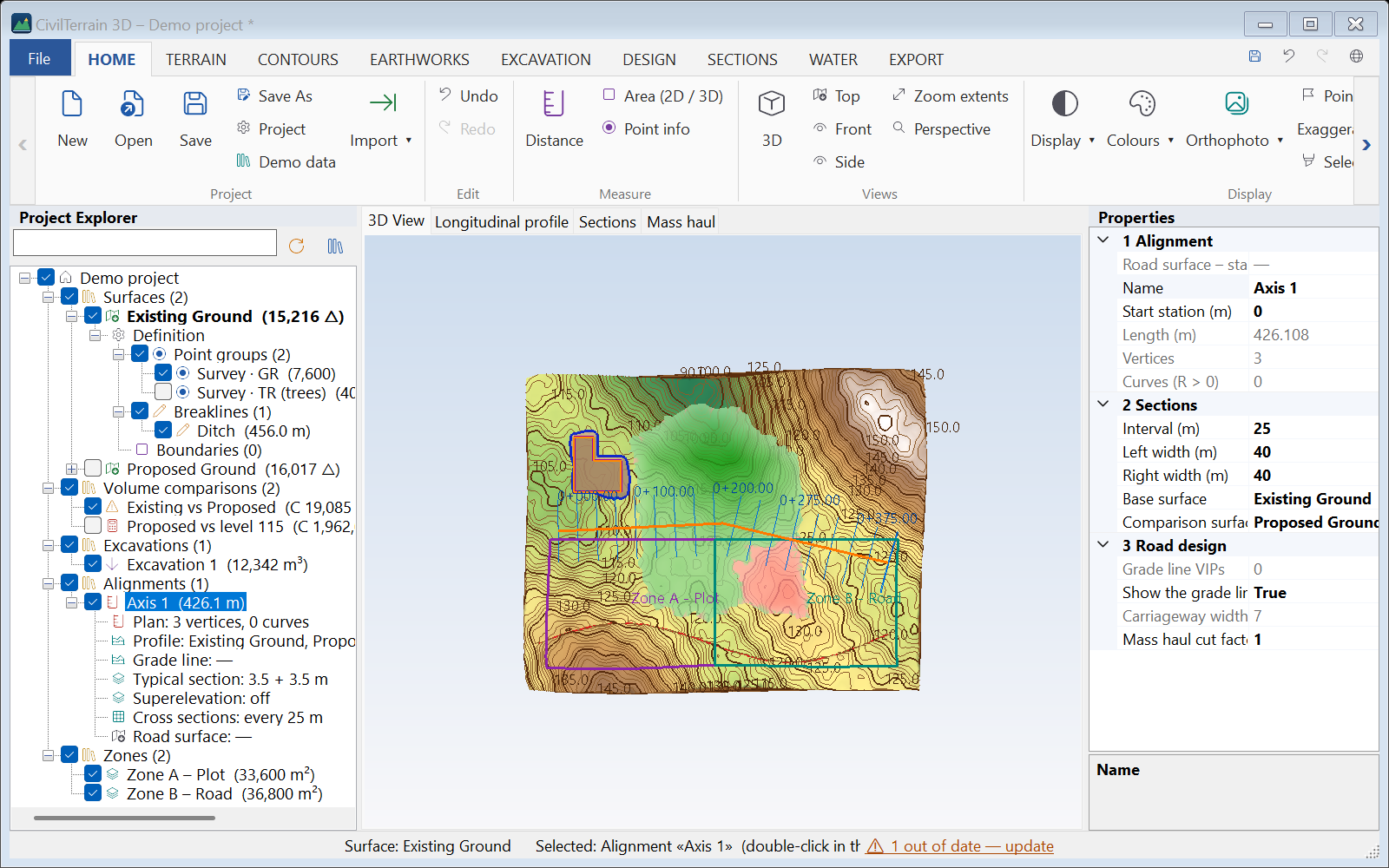
Below every alignment are its parts, each with a short summary:
- plan (vertices, curves);
- profile (surfaces);
- grade line;
- typical section and typical sections along the axis;
- superelevation;
- cross sections;
- depth lines;
- road surface.
Double-click a part to open its window, e.g. “Grade line” opens the grade line, while “Road surface” builds or updates it.
Out of date and dependencies
When a surface changes, whatever is computed from it updates automatically: comparisons, excavations, polygon earthworks, building-code checks, section grids. Automatic update can however be switched off in the Properties. The road surface is also built by a command. In these cases the object is marked ⚠ out of date:
- with an icon in the tree;
- with an explanation when you hover over it;
- in the Properties (State);
- in the status bar, as a link “⚠ N out of date — update”.
The same holds for a road surface if the alignment, grade line, typical section, superelevation or ground changed after it was built.
- Update: right-click → Update on one object, or the Update all button above the tree, or click the message in the status bar.
- ⚠ surface missing: a surface the object is computed from was deleted.
- Used by: the Properties of every surface (and its tooltip in the tree) list the objects that use it. When a surface is deleted, the program names them before asking for confirmation.
Item list
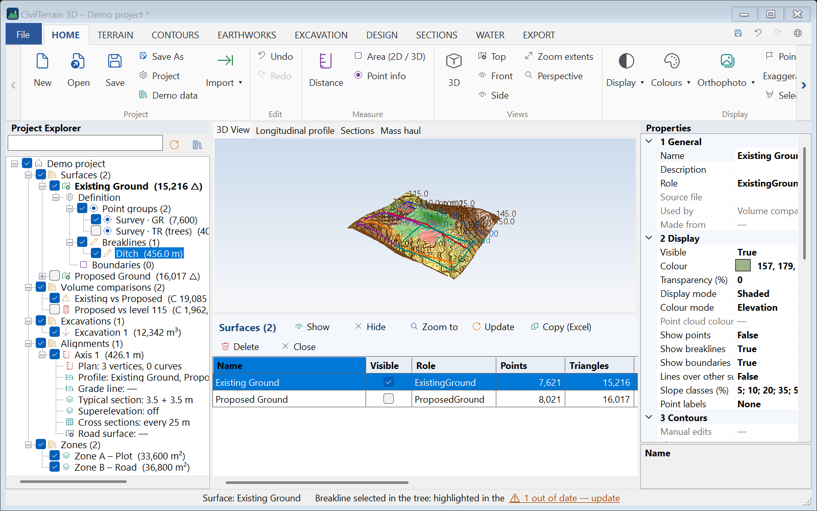
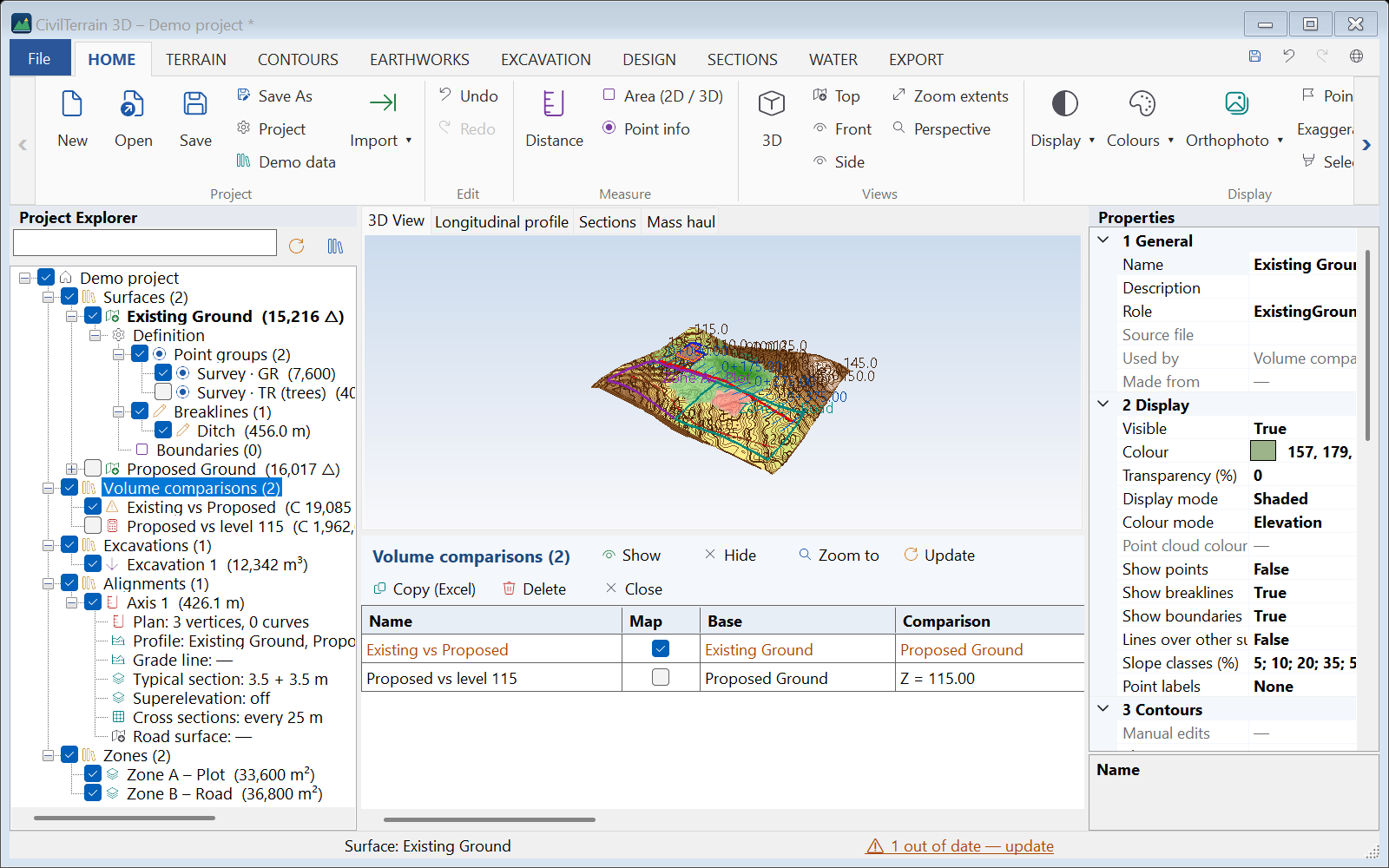
Clicking a collection, e.g. Surfaces, opens the item list under the 3D view, a table with the key figures of every object:
- surfaces: points, triangles, Z min/max, area, maximum edge, what uses them;
- comparisons: base, comparison, cut, fill, net volume, state and centroids (X, Y, Z of the cut and of the fill, CG distance); polygon earthworks have the centroids too;
- alignments: length, stations, curves, grade line, road surface etc.
Working with the table:
- click a header to sort;
- rename in place (F2);
- the check box shows or hides;
- with several rows selected: Show, Hide, Zoom to, Update, Copy (Excel) and Delete (one question for all).
Objects that are out of date are shown in orange. Selecting a row also selects the object in the tree. Clicking the project itself shows a summary of every collection.
Many feature lines
Up to 500 feature lines are shown one by one under Feature lines. With more (e.g. a network of routes from a DXF, section 15.7), the tree groups them per code / layer, with their count and length, e.g. “ROADS (1,250 lines, 84.3 km)”. When you open the node of a layer, its first 300 lines appear, followed by a “… and N more (Item list)” node. The check box of the node shows or hides every line of the layer. A line you select in the drawing or in a table is added to the tree and selected. Right-click Feature lines: Weighted slope of all lines… and Import routes (DXF / DWG)….
Selecting by clicking in the drawing
A plain click in the 3D view (without dragging) selects the object under the cursor, in this order:
- lines and outlines (alignments, feature lines, excavations, zones, polygons, building-code checks, section grids, spot grids, breaklines);
- the area the point is in, or a marker of a spot grid (section 5.4);
- the cut / fill map.
Its node is selected in the tree and its Properties open, as in a CAD program. A click on bare terrain changes nothing (the active surface stays the same; surfaces are selected in the tree). Drawing tools, the double-click that ends a line and the vertex / edge / triangle selection are not affected. If the object is hidden by the search, its name is shown in the status bar.
3.3 Theme
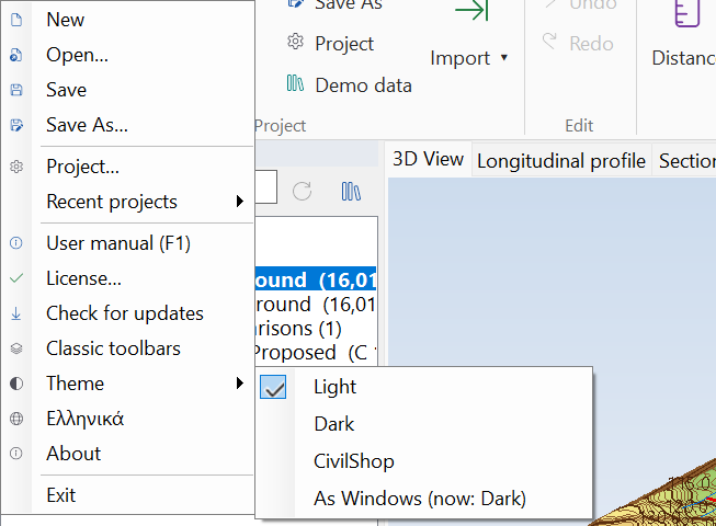
In File → Theme you choose how the program looks. The choice is remembered.
| Theme | Description |
|---|---|
| Light | The default. It looks the same as earlier versions. |
| Dark | Dark windows, ribbon, tree, tables and drawings (profile, cross sections, mass haul diagram) with light text, and a dark background in the 3D view. It suits long working hours or low light. Available on Windows 11. |
| CivilShop | Light, in the CivilShop colours: a dark title bar and tab strip, a yellow line under the selected tab and blue headings. |
| As Windows | Dark or light, following the Windows setting for apps (Settings → Personalization → Colors). The menu shows which of the two applies now. On Windows 10 it stays light. |
The theme changes when the program restarts. After you choose a theme, the program asks whether to restart now. If the project has unsaved changes, it first asks you to save them, and then opens the project again. If you answer “No”, the new theme applies at the next start. With “As Windows”, a message in the status bar tells you when the Windows setting changes while the program is open.
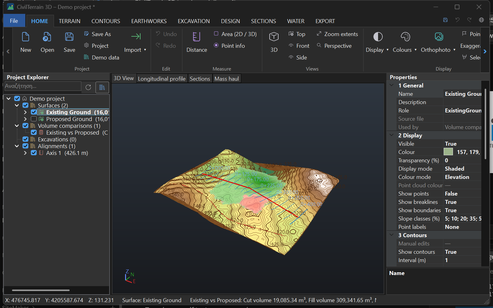
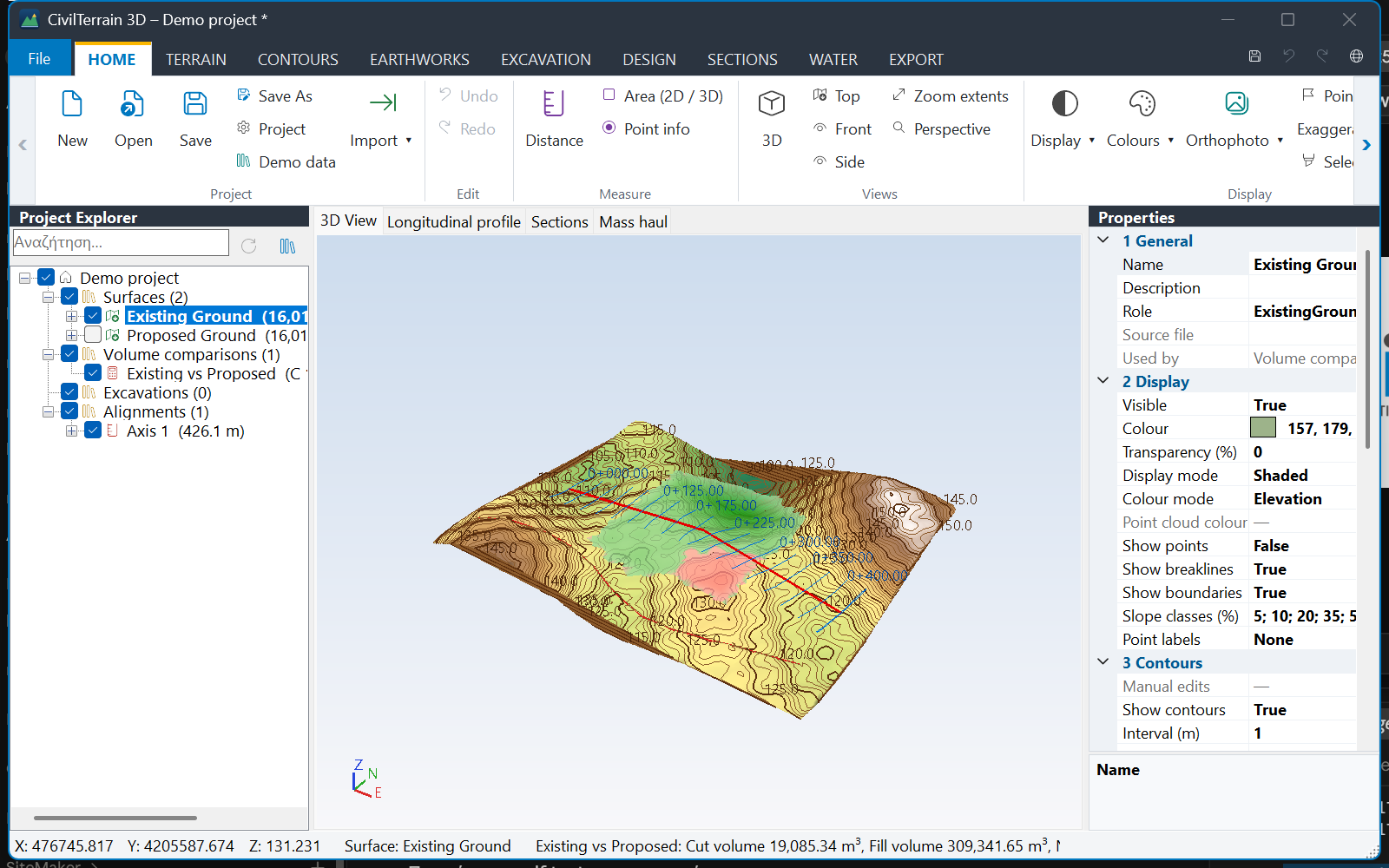
The File → About window shows the version and a link to the CivilShop store. The CivilShop logo appears there and on the start screen.
4. 3D navigation and display
| Action | Control |
|---|---|
| Orbit | Drag with the left mouse button |
| Pan | Drag with the right or middle button, or Shift+left |
| Zoom | Mouse wheel — zooms towards the point under the cursor |
| Views | 3D, Top, Front, Side, Zoom extents |
| Projection | Perspective or Orthographic (toggle with the same button) |
4.1 Display modes and colouring
From HOME → Display: Shaded, Wireframe, Shaded + Wireframe, Points. From Colours: Elevation colours (hypsometric ramp), Slope analysis, Solid colour. Settings apply to the active surface; details (colour, transparency, slope classes) are in Properties.
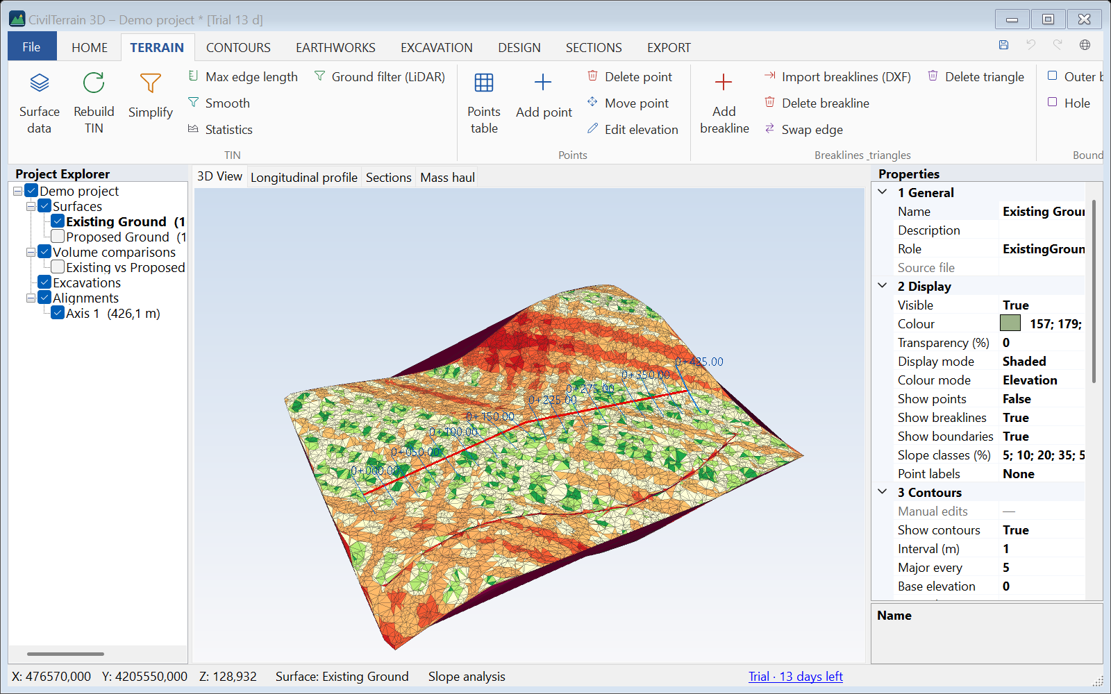
Slope classes (e.g. 5; 10; 20; 35; 50; 100 %) are defined in the surface Properties. Vertical exaggeration (×1 to ×10) stretches the display only, not the data. Transparency lets you see two surfaces at the same time. With Lines over other surfaces (Properties → Display) the triangles, contours and lines of a surface also show where another surface lies above them (e.g. the surface of the points of a spot grid, section 5.4); while such a surface is not the active one, the pointer reads the elevations of the surface below it. A Duplicate of a surface keeps this option; the other surfaces made from it (merge, smoothing, simplification and so on, section 5.4) start without it.
4.2 Selecting vertices, edges, triangles
From HOME → Select choose Vertices, Edges or Triangles and click on the active surface. The status bar shows coordinates, 2D/3D lengths, slope and areas. Esc clears the selection.
5. Measurements, points and spot grid
5.1 Measurements
On HOME → Measure:
| Tool | Result |
|---|---|
| Distance | Draw a polyline (2 or more points). Gives horizontal length, slope length, length on the surface (following the terrain), ΔZ, average grade and azimuth (grad) for 2 points. |
| Area (2D / 3D) | Draw a closed polygon. Gives plan area, perimeter, the true 3D surface area and min / mean / max elevation. A warning appears if part of the polygon lies outside the surface. |
| Point info | Click points (repeating): X, Y, the Z of every visible surface, the slope at the point and the WGS84 geographic coordinates. |
Results are collected in the Measurements window and can be copied (Copy) to Word or Excel.
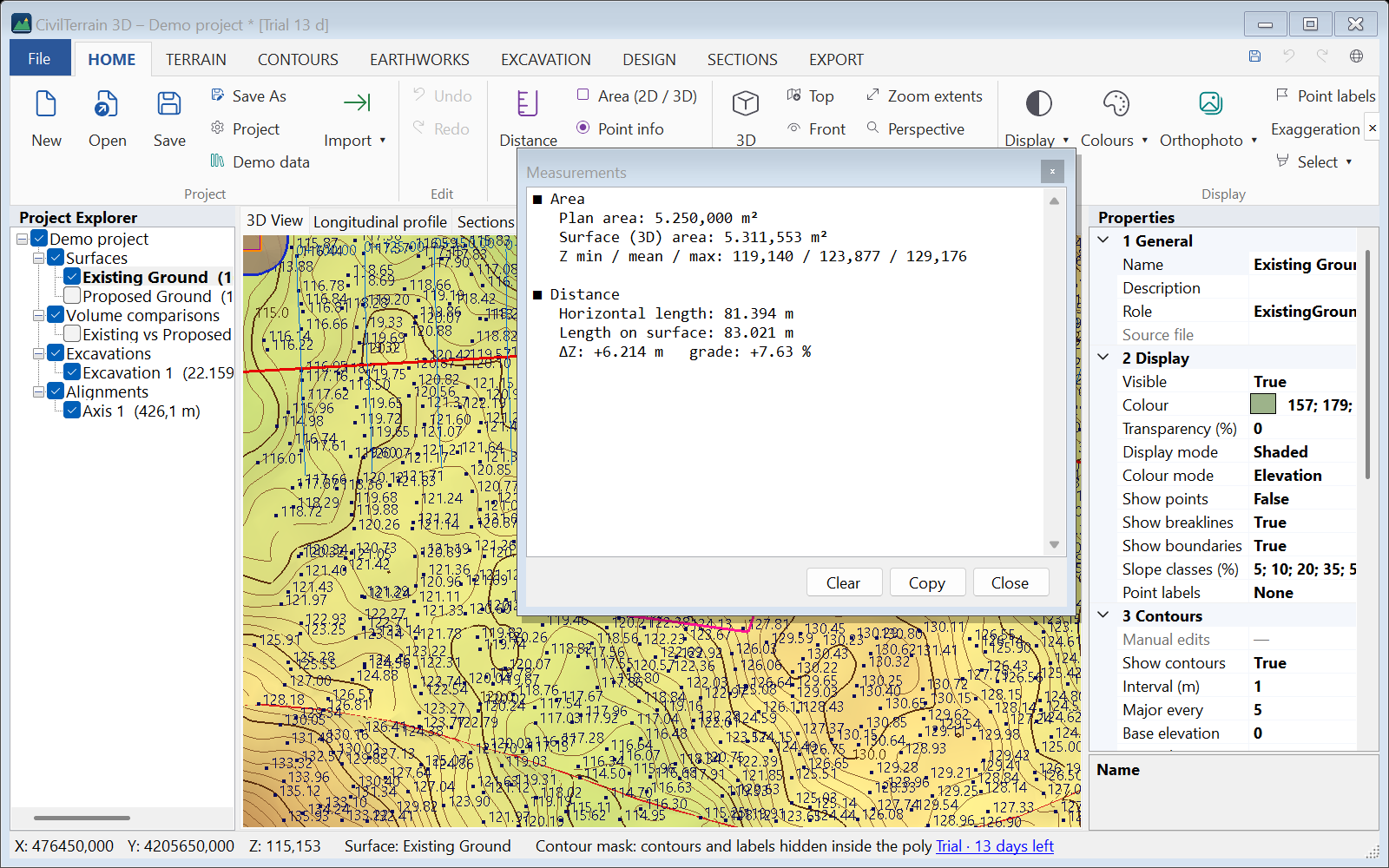
5.2 Point labels
HOME → Point labels (or Properties → Display → Point labels): None, Number, Elevation, Number + elevation. The number is the point id from the CSV/TXT file ("No." column). In dense areas only the labels that fit are drawn — zoom in to see more.
5.3 Points table
TERRAIN → Points table lists every point of the active surface by group, even for millions of points (virtual list).
- Search by point number or group name.
- Edit X, Y or Z directly in the cell — the surface updates immediately and the change can be undone with Ctrl+Z.
- Double click or Zoom to: the drawing moves to the point.
- Delete selected and Export CSV.
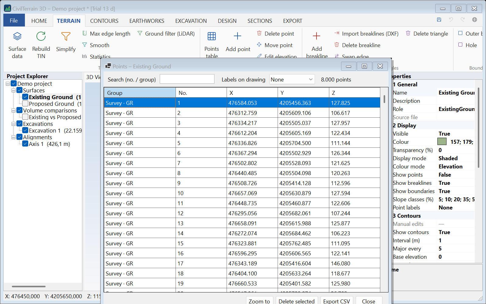
5.4 Spot grid
A spot grid gives points every so many metres (e.g. every 5 m) inside a perimeter, with the elevation of the surface at each point. The points are numbered (S1, S2 …) and shown in the view with a marker and a label, e.g. “48.62 m”, on the surface or on the orthophoto. Use it for the spot elevations of a layer once it is laid (checking, measurement, as-built survey), for setting out, and to check a drone survey against the design: with a second surface every point also gets its Δz.
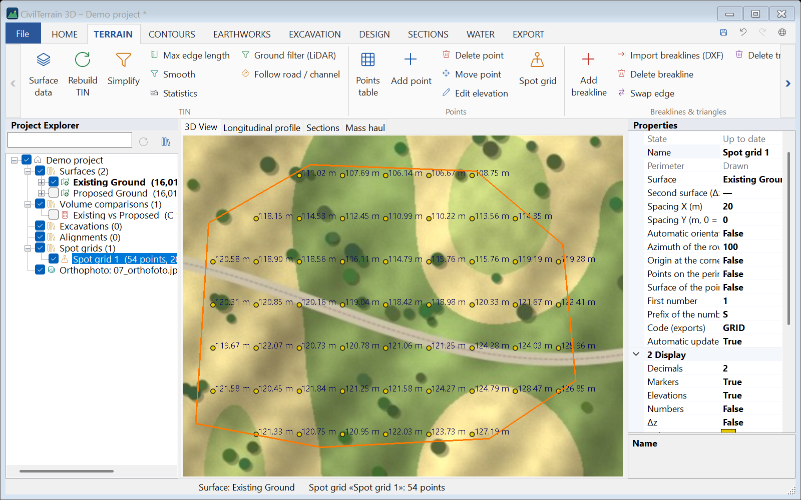
- Make the surface active (e.g. the drone survey). If the perimeter already exists, select it in the tree: a zone, a closed line, the outline of polygon earthworks, a grading optimization, a sloped design, a building-code check or a section grid, a closed breakline or a boundary.
- TERRAIN → Points → Spot grid. The selected outline becomes the perimeter. Otherwise you choose where it comes from: Outline of the surface «…» (the whole survey; the default), Click an existing outline (zone, closed line, breakline, boundary, excavation), Draw the polygon, From a DXF / DWG or Type / paste coordinates.
- In the New spot grid window set the spacing and the other settings (table below) and press Create.
When a spot grid is selected in the tree, the same command opens its window to edit it. The table and the exports of a grid open from its menu in the tree (right click, below); the exports also from EXPORT → Points → Spot grid.
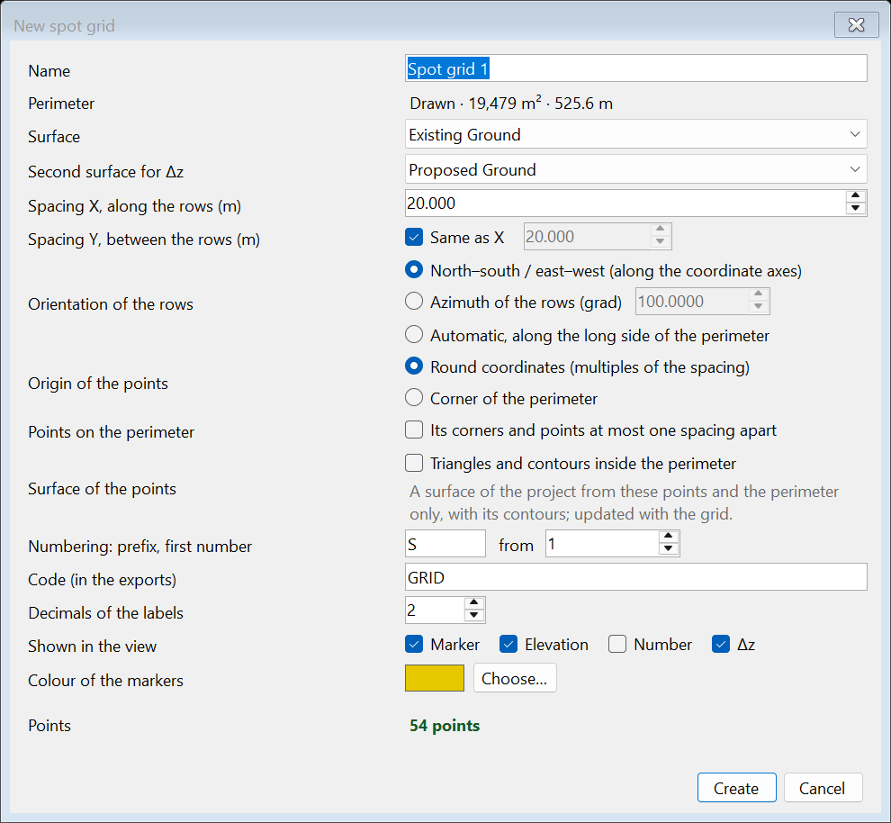
| Setting | Description |
|---|---|
| Name | The name of the outline it comes from is proposed (a zone, a line …), otherwise “Spot grid N”. |
| Perimeter | Where it came from, its area and length. When editing, New perimeter… takes it again (from the same sources) and comes back to the window. |
| Surface | The surface that gives the elevation Z of the points. The active one by default. |
| Second surface for Δz | Optional (“— none —” by default). Every point also gets its elevation Z2 and the difference Δz = Z2 − Z: positive = fill, negative = cut. |
| Spacing X, along the rows (m) | The distance between the points of a row. The first grid proposes a spacing for about 2,000 points; the next ones start from the settings of the last one. |
| Spacing Y, between the rows (m) | Same as X (default) or another value, for a rectangular grid (e.g. 10 × 5 m). |
| Orientation of the rows | North–south / east–west (along the coordinate axes, default); an Azimuth of the rows (grad) that you type (100 = west to east); or Automatic, along the long side of the perimeter, e.g. for a platform or a road that is not parallel to the axes. |
| Origin of the points | Round coordinates (multiples of the spacing, default): the points fall on the same positions in every survey. Or the Corner of the perimeter. |
| Points on the perimeter | Adds points at the corners of the perimeter and along it, in equal parts not longer than the spacing. They are numbered after the grid points. A point of the perimeter (a corner too) closer to a grid node than 2% of the spacing, and at most 5 cm, is that node and is not added twice (e.g. a side a few centimetres off a row of a 5 m grid). |
| Surface of the points | Triangles and contours inside the perimeter (off by default): makes a surface of the project from the points of the grid and the perimeter only, with triangles up to the perimeter and never outside it, and their contours (below). It adds no points to the exports. |
| Numbering: prefix, first number | Prefix S from 1 by default: S1, S2 … |
| Code (in the exports) | The point code in the CSV, TXT and Excel files (GRID by default). |
| Decimals of the labels | Decimals of the elevation and Δz in the view, in the DXF / DWG and on the plan of the PDF (0–4, default 2). The tables and point files always have 3 decimals. |
| Shown in the view | Marker and Elevation (ticked), Number, and Δz when there is a second surface. The same labels are written on the plan of the PDF. |
| Colour of the markers | Yellow by default; Choose… for another colour (the view only). |
| Points | How many points the settings give, as you type. Above 250,000 the number turns red, the window says “Too many points (more than 250,000): increase the spacing.” and the grid is not created. |
In the view
Each point is shown with a round marker in the colour of the grid and, to its right, its elevation (e.g. “48.62 m”), with the number above and Δz below (red in cut, blue in fill). The perimeter is drawn on the surface. As many labels are written as fit without overlapping one another or the markers of the labelled points: every few rows and columns from far away, more densely as you come closer (in perspective, near points more densely than far ones). Zoom in to see every label. Where the points crowd on the screen (far away, or the far part of an oblique view) the markers become small, faint dots, so that the ground shows through. The markers are drawn over the surface, so in an oblique view they also show behind hills.
The grid goes into the tree, in the Spot grids collection, with its number of points and spacing (and “with surface” when it has a surface of the points) and a check box to show / hide it. A click in the view on its perimeter, on one of its markers (where they stand apart) or inside it selects it; if it was made from a zone, the line and the inside select the zone and a marker the grid. Creating it, editing it in its window and deleting it are undone with Ctrl+Z. Right click: Edit…, Table…, Export…, Surface of the points (turns the option on or off), Go to the surface of the points (when there is one), Recalculate, Delete. In the Properties you change the same settings (a spacing that would give more than 250,000 points is refused), the Surface of the points too, and see the results: points of the grid / on the perimeter, points off the surface, Z and Δz min / mean / max, points in cut / fill / no change, direction of the rows, area and length of the perimeter and, with the surface of the points, its triangles.
The points table
Right click on a grid in the tree → Table… shows its points: No, Point, X, Y, Z, with a second surface also Z2, Δz, and Code. Above it you see how many points there are (of the grid and on the perimeter) and the range of Z. The numbers are in the number format of Windows (e.g. a decimal comma with Greek regional settings), so that they paste into Excel as numbers.
- Double click or Zoom to: the view goes to the point and marks it with a cross; its coordinates are shown in the status bar.
- Copy: the selected rows, with the column headings, to paste into Excel; all the rows when one row or every row is selected. Ctrl+C copies just the selected rows, even a single one.
- Export…: as below.
The table stays open beside the drawing and is updated when the grid is computed again; the rows you are looking at stay in place.
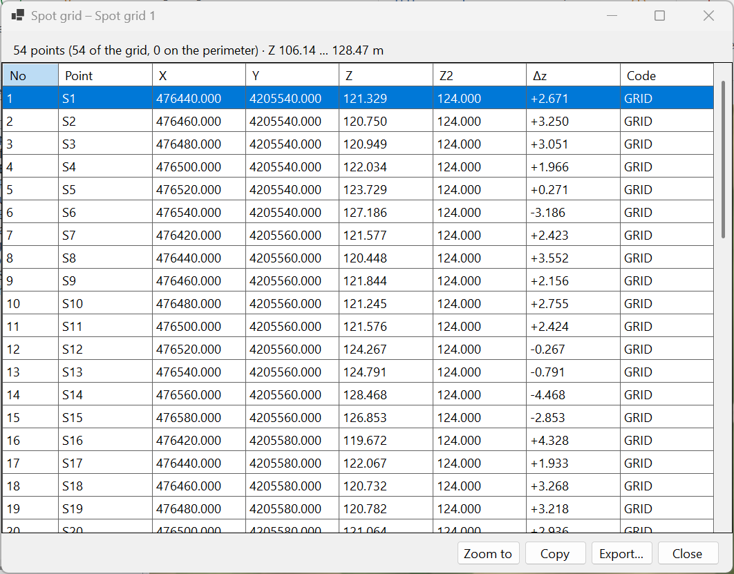
Exports
Right click on the grid in the tree → Export…, the Export… button of the table, or EXPORT → Points → Spot grid (for the grid selected in the tree, otherwise the one in the open table or the last one). A save window opens and the file type sets the format. If the grid is out of date, it is computed first. Excel and PDF files open as soon as they are saved.
| Format | Content |
|---|---|
| CSV | Columns PT,X,Y,Z,CODE (with a second surface also Z2,DZ), 3 decimals with a decimal point, commas between the values. It reads back into the program with the point numbers. |
| TXT (PNEZD) | Number, northing (Y), easting (X), elevation, code, separated by spaces, with no header — for setting-out instruments and software. |
| DXF / DWG | Layers SG_BOUNDARY (perimeter), SG_POINTS (points at their elevation), SG_MARKER (cross), SG_NUMBER (number), SG_ELEV (elevation) and, with a second surface, SG_DZ. Markers and texts are in plan. A DWG is written for up to 50,000 points; above that the program suggests DXF (the same layers, in seconds) or CSV. |
| Excel | A Summary sheet (project, surfaces, perimeter, spacing, direction, origin, count, numbering, Z and Δz) and a Points sheet (No, Point, X, Y, Z, Z2, Δz, Code). With the surface of the points, the summary also gives its name, its triangles and the contour interval. |
| A summary with the method, the plan on A3 at a standard scale (1:N with a scale bar, contours, perimeter, points and labels where they fit) and the list of points on A4, two lists per page, with Δz in red / blue. The list is written for up to 10,000 points; above that, see the CSV or Excel file. With the Surface of the points on, the contours of the plan are those of that surface. |
Surface of the points: triangles and contours
With the option Triangles and contours inside the perimeter of the window (row Surface of the points), or Surface of the points in the Properties and in the grid's menu in the tree, the points of the grid become a surface of the project, e.g. “Grid 20 m – surface”: a TIN of the grid points and the points of the perimeter only, with triangles up to the perimeter and never outside it, and its contours, also only inside the perimeter. Outside the perimeter the survey shows as before. By default no surface is made: a grid gives points only, as before.
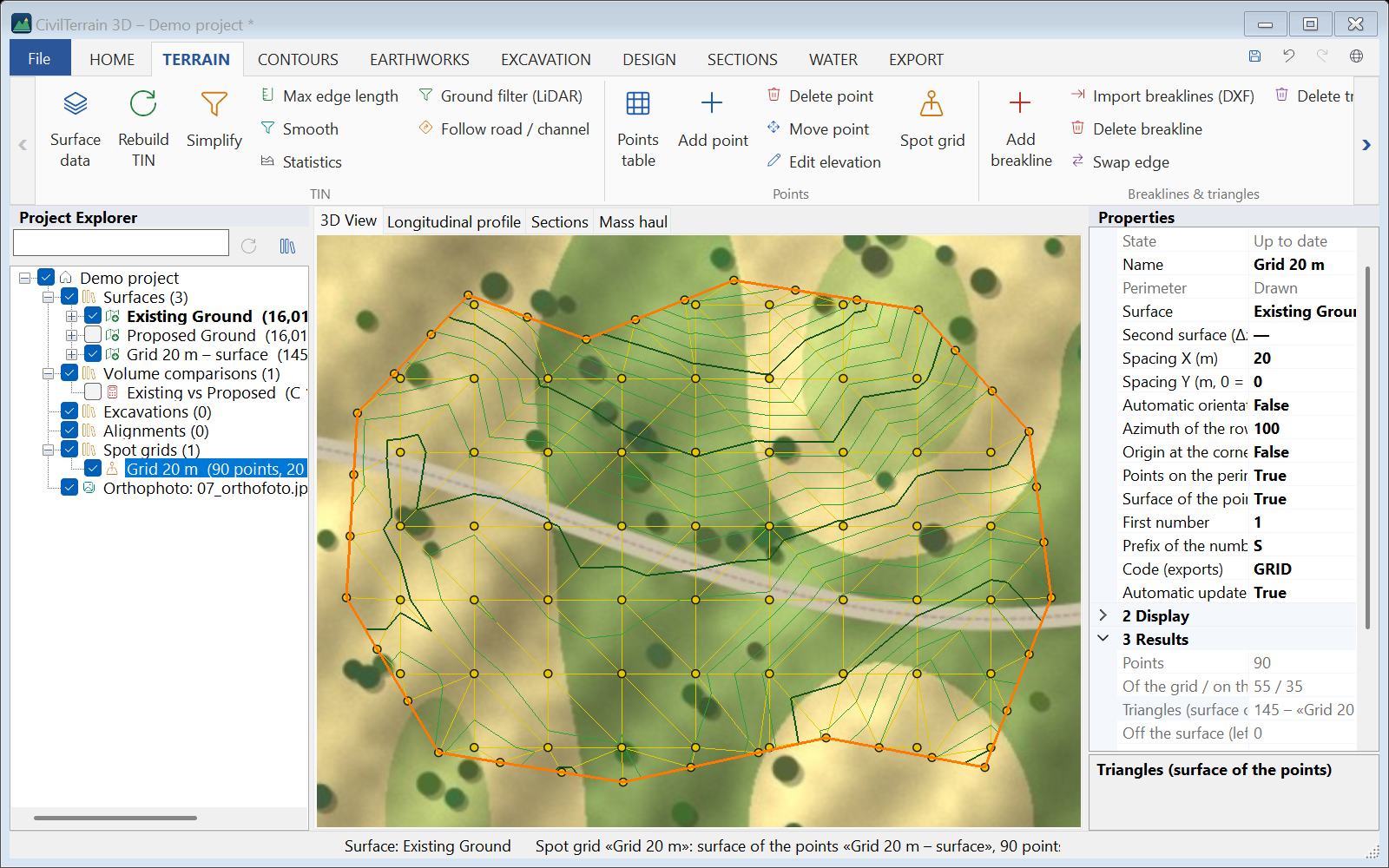
- The surface shows as a wireframe in the colour of the grid's markers, with green contours at the interval of the grid's surface. It is drawn over the other surfaces (surface Properties → Lines over other surfaces), so that it shows whole over the survey or the orthophoto; in an oblique view it also shows behind hills. While it is not the active surface, the pointer reads the elevations of the surface below it. Colours, interval and labels change in its Properties.
- Every point of the grid is a vertex of the surface, with its number (S1, S2 …). On the perimeter, besides the grid points that lie on it, the surface takes the elevations of the grid's surface at its vertices and at most one spacing apart. With Points on the perimeter these are set-out points too; without them they go into the surface only, not into the exports.
- Where the perimeter leaves the grid's surface (there are no grid points and no elevations there), the triangles stop at the last grid points and at the pieces of the perimeter that lie on the surface; no triangle goes outside the perimeter. Where the grid's surface has a hole inside the perimeter, the triangles join the points around it.
- A perimeter with many small vertices (e.g. the outline of a survey) gives many thin triangles along it and takes a few seconds; for a cleaner result draw a perimeter with few vertices.
- It is an ordinary surface (role “Other”): contours and TIN to DXF / LandXML, volume comparisons, sections (while visible it also shows in the profiles and sections of alignments). In its Properties, Made from names the grid. In the grid's PDF export the plan shows its contours.
- It is linked to the grid: it is made again with it (a change of the grid's surface, the perimeter, the spacing, the numbering and so on), only when the points change, and not when the project opens. When you rename the grid, the surface is renamed too, as long as it keeps the name the program gave it.
- Its data are made from the grid and cannot be edited: the commands that change the data of a surface (e.g. the terrain tools, Surface data, the ground filter, adding data to the active surface, following a road) say so in a message and change nothing: most of them before their window opens, the imports as soon as you choose “Add to the active surface”, Replace terrain and Remove objects as soon as you choose “In the same surface” (in a copy they work as usual). To edit it, make a Duplicate first: the duplicate keeps the look (wireframe, lines over other surfaces), becomes the active surface and can be edited as usual. The other surfaces made from it are ordinary surfaces, without “Lines over other surfaces”: a merge, a smoothing, a simplification, an elevation offset, objects removed or terrain replaced in a copy, and the “Surfaces inside the perimeter” (section 12.6).
- When you turn the option off or delete the grid, the surface is removed (if another object uses it, e.g. a volume comparison, the program asks first); Undo brings it back. If you delete the surface, the grid's option is turned off.
- A grid cannot take its elevations (or Δz) from its own surface of the points, not even through another grid; another grid can. If an undo brings back such a source, the grid's node says “⚠ surface of the points not updated” until you change the source.
- Versions up to 1.6.13 open the project and show the surface as an ordinary surface, not linked to the grid.
Updates and numbering
- When the surface or the second surface changes (an edit, remove objects, new data), the grid is computed again by itself. With Automatic update off in the Properties it is marked ⚠ out of date (section 3.2). The project saves the settings of the grid; the points are computed again when the project opens.
- The numbers follow the geometry only: row by row from the origin side (with north–south orientation, from the south-west) and then the perimeter points. So every point keeps its number when the surface changes. The numbers change only if you change the perimeter, the spacing, the orientation, the origin, the perimeter points or the first number.
- A point inside the perimeter but off the surface is left out together with its number, and the program says how many were left out. A point off the second surface is kept without Δz.
6. Project and coordinate system
A project (.ct3d) contains all surfaces with their data (points, breaklines, boundaries, edits), volume comparisons, excavations and alignments. Coordinates are stored at full precision.
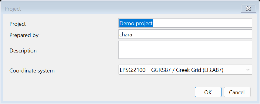
In File → Project… set the name, author, description and the coordinate system (default GGRS87 / Greek Grid). These appear in the reports.
7. Importing data
All imports are under HOME → Import ▾. Data go into a new surface or, with Add to the active surface, into the surface already selected (e.g. to add breaklines or a second point file).
After every import the Surface data dialog opens (section 9.2) so you choose what takes part before the TIN is built. Points are organised in groups: per code (CSV/TXT), per layer (DXF) or per file (LAS). Points and vertices with invalid coordinates (e.g. “nan” or “1e400” in the file, or out of the coordinate transformation) are left out of every surface import and of “Level from 3D polyline”, and a message says how many before the dialog opens; if no valid point is left, nothing is imported.
7.1 CSV / TXT / XYZ
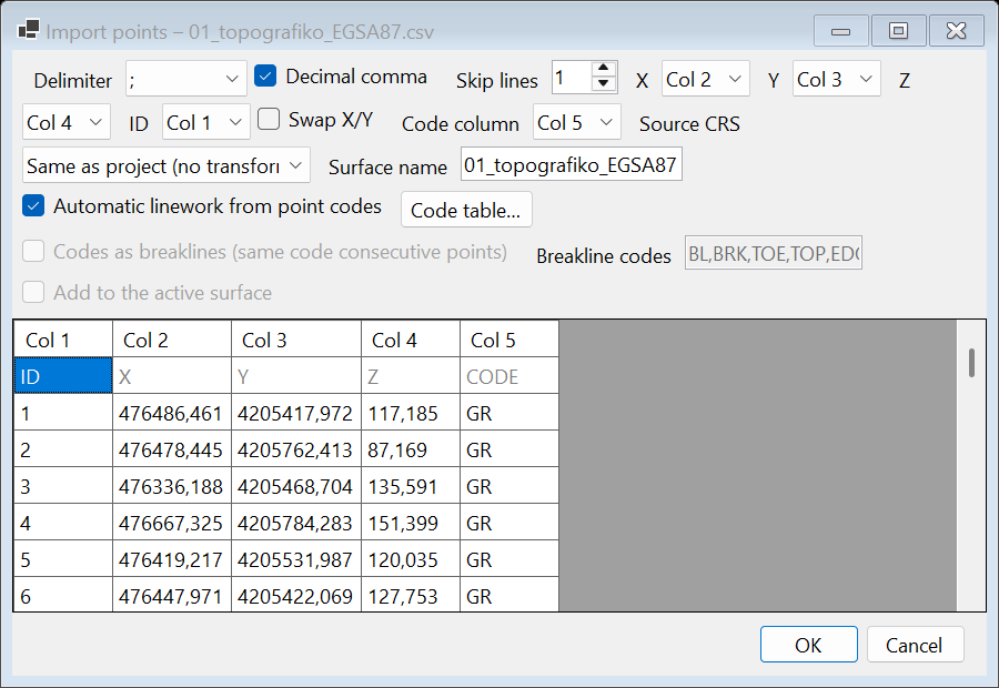
The delimiter (comma, semicolon, tab, space), decimal comma, header lines and the X, Y, Z, ID and code columns are detected automatically. Check the preview and correct if needed:
- Skip lines: header lines (shown grey).
- Swap X/Y: for files ordered Northing, Easting.
- Source CRS: if the points are in another system than the project (e.g. WGS84) they are transformed automatically.
- Codes as breaklines: consecutive points whose code starts with one of the breakline codes (e.g.
BL, BRK, TOE, TOP, EDGE) are joined into a breakline.
7.2 DXF
POINT, LINE, LWPOLYLINE, POLYLINE (2D/3D/polyface) and 3DFACE entities are read from ASCII DXF of every version. In the dialog choose the layers and whether POINTs become points, polyline vertices become points, 3D polylines become breaklines and 3DFACEs a fixed TIN. 3D polylines with a spline fit are read by the points of their fitted curve; the control points of the spline frame are ignored.
With 3D polylines as 3D lines only (no surface) no surface is made and the Surface data dialog does not open: every polyline of the chosen layers becomes a 3D line of the project (e.g. a route), and one click on it shows its weighted slope (section 15.7). In the normal import the option is not ticked at first: as before version 1.6.13, a drawing of 3D polylines is made into a surface. The program remembers your choice in this window and, if you ticked it, ticks it again when the drawing has 3D polylines with elevations and no POINT or 3DFACE. The remembered choice changes only when you tick the option or import such a drawing; another drawing (e.g. a survey with points) made into a surface does not change it. SECTIONS → Route → Import routes… always imports without a surface. When the option is ticked:
- the surface options (points, vertices, breaklines, 3DFACE, surface name, add to the active surface) are unticked and disabled; they come back as they were when you untick it;
- layers without any polyline with elevations (e.g. a frame or a title block) start unticked when another layer has routes; you can tick them again;
- files in longitude / latitude or Web Mercator are transformed into the project's system; in an empty project, the projected system of the file (e.g. GGRS87, UTM) that you set in Source CRS becomes the project's system;
- if the coordinates look like degrees (longitude / latitude) while Source CRS is “Same as project”, a warning appears; the lines are already imported: undo (Ctrl+Z), choose WGS 84 (lon/lat) in Source CRS and import again. A local drawing in metres near 0, 0 (e.g. a 150 × 80 m yard) does not give the warning;
- vertices with invalid coordinates (e.g. “nan” in the file) are skipped, and the import message says how many;
- the whole import is undone with one Undo.
The Contents line of the dialog also shows how many polylines have elevations, e.g. for the sample 13_diadromes.dxf “0 POINT, 11 polylines (10 3D), 0 faces”: the 10 routes and a 2D frame.
7.3 LAS / LAZ (point clouds)
LAS 1.0–1.4 is supported. The dialog shows point count, extent and EPSG. Options: Ground only (class 2), Leave out noise (classes 7 and 18 – e.g. birds, reflections), keep every N-th point, grid thinning (keeps the lowest point per cell – suitable for ground) and Gridded surface in the RGB colours of the cloud (section 8.3). LAZ requires the free laszip64.exe in the program's tools folder or on the PATH. If the import fails (e.g. a LAZ file without laszip64.exe, or a file that is not LAS), the program says why; if the chosen classes leave no point, it says “No points with the selected classes.”
7.4 PLY / OBJ, LandXML
- PLY/OBJ: with triangles they are imported as a fixed mesh, otherwise as points.
- LandXML: TIN surfaces (points and faces), breaklines, CgPoints and EPSG.
- DEM (GeoTIFF, ASCII Grid, SRTM, BIL / FLT): section 7.6.
7.5 Point codes – automatic linework
When the CSV/TXT file has a code column, points with the same code are joined automatically into lines. In the import dialog tick Automatic linework from point codes.
| Field code | Result |
|---|---|
ΚΡ1, ΚΡ2 | Points of each code are joined in file order; the number keeps parallel lines apart (e.g. two curbs). |
ΚΡ1 B (or ΑΡ) | Begin a new line. |
ΚΡ1 E (or ΤΕ) | End the line. |
ΚΤ C (or ΚΛ) | Close to the first point (buildings). |
The code table (DESIGN → Code table or the button in the import dialog) defines for each code: whether it forms lines, whether they are terrain breaklines, whether its points take part in the surface (e.g. not buildings, trees) and the colour. Greek field codes (ΚΡ, ΑΞ, ΑΣ, ΦΡ, ΠΟ, ΤΑ, ΡΕ, ΤΟ, ΠΕ, ΚΤ, ΔΕ) are predefined; the table is kept for all projects.
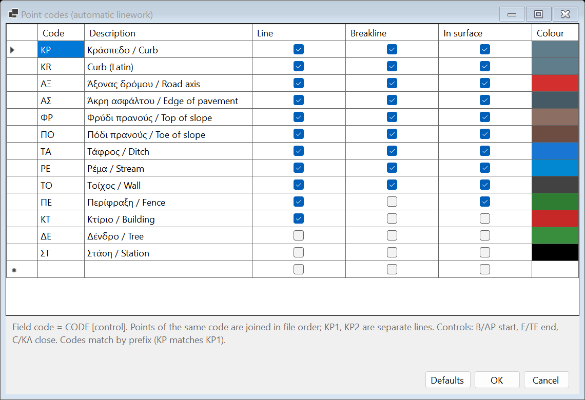
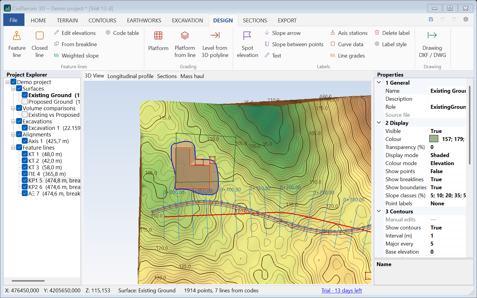
The lines become project feature lines (see "Feature lines and platforms"); those marked as breaklines also enter the TIN. Sample: 08_kodikopoiisi.csv.
7.6 Digital elevation models (DEM)
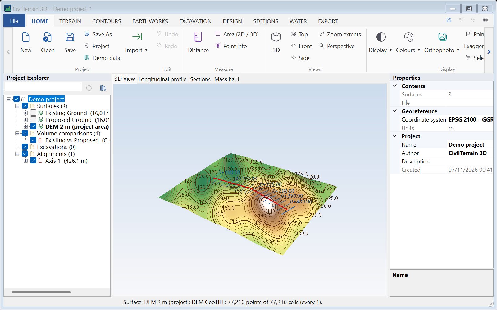
HOME → Import → DEM (GeoTIFF, ASC, HGT, BIL)… reads gridded elevations and turns them into a surface (a fixed triangle mesh, one point per cell). Cells without a value (NoData) stay empty.
| Format | Files | Notes |
|---|---|---|
| GeoTIFF | .tif, .tiff | Classic TIFF and BigTIFF (over 4 GB), in strips or tiles (also Cloud Optimized GeoTIFF); LZW, Deflate, PackBits compression; 8–64 bit integer or floating point values; NoData and value scale / offset. Georeference from the GeoTIFF tags or from a world file (.tfw). |
| ESRI ASCII Grid | .asc | Header ncols, nrows, xllcorner / xllcenter, cellsize, NODATA_value. An .asc chosen in the point import is recognised as a DEM automatically. |
| SRTM / NASADEM | .hgt, .hgt.zip | 1″ (≈30 m) or 3″ (≈90 m) tiles; the position is read from the name (e.g. N38E023.hgt), WGS 84. |
| ESRI BIL / FLT | .bil, .flt with .hdr | Binary rasters with a header, as most GIS export them. |
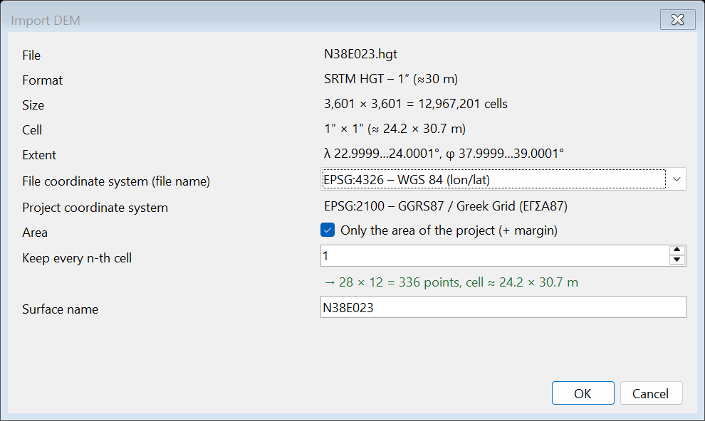
The dialog shows the format, size, cell and extent of the file and sets:
- File coordinate system: read from the file itself, from the
.prjnext to it or from the name of the SRTM tile (the source is shown in brackets). When it differs from the project's system the points are transformed — e.g. a DEM in WGS 84 degrees goes into GGRS87. For the first DEM of an empty project you also choose the project's system. - Only the project area: from a large DEM (e.g. a 1° × 1° tile) only the area of the project's surfaces, alignments and zones is kept, with a margin. It is selected automatically when the DEM is much larger than the project.
- Keep every n-th cell: thinning for very large DEMs. The number of points and the resulting cell are shown; the suggested value keeps up to 4 million points (16 million at most).
- File without georeference: you give the cell size and the lower-left corner.
Large files are read row by row without loading the whole file into memory, so choosing an area or thinning also makes the import faster.
8. LiDAR / drone point clouds and orthophotos
8.1 Ground filter
Unclassified drone or LiDAR clouds contain vegetation, buildings and vehicles. The ground filter (progressive morphological filter) separates them from the ground:
- When a LAS file is imported without class filtering the program offers to run the ground filter, or later: TERRAIN → Ground filter (LiDAR).
- Adjust the parameters (the defaults suit most cases).
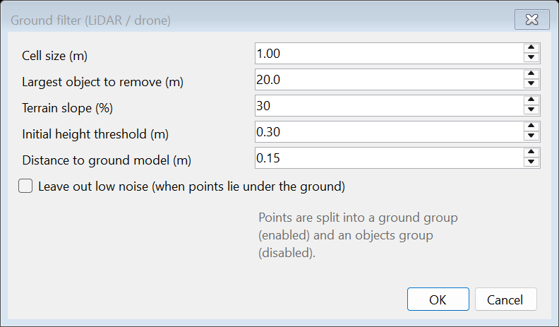
- Points are split into a "ground" group (enabled) and an "objects" group (disabled) and the TIN is rebuilt. Any group can be re-enabled from Surface data.
| Parameter | Meaning |
|---|---|
| Cell size | Density of the helper grid (≈ average point spacing, e.g. 0.5–1 m); “Leave out low noise” needs about one point per cell or more. |
| Largest object | The widest building/tree to remove (e.g. 20 m). |
| Terrain slope | Maximum expected slope of the natural ground. Larger for mountainous areas. |
| Initial height threshold | Height above "ground" already treated as an object (e.g. 0.3 m). |
| Distance to ground model | Final tolerance: points closer to the ground model than this are kept as ground. |
| Leave out low noise | For clouds with points under the real ground (reflections, multipath), which otherwise leave pits in the ground model. Single points or small groups (up to about 3 m across) more than 0.5 m + terrain slope × cell size under the ground around them (0.8 m with the defaults; cells under 1 m count as 1 m) are left out of the ground; long low ground (ditches, channels, streams) stays. The box is not ticked by default: the filter works as up to version 1.6.13. Your choice is kept for the next time and also applies to the general filter of Follow road / channel (section 8.4). See the limits below. |
- real pits narrower than about 3 m and deeper than the threshold (0.8 m with the defaults), e.g. a manhole: they are bridged;
- narrow ditches and channels in a sparse cloud (few points per m²) or broken by crossings every few metres: they may be filled in part or even whole; for a channel with water, where only a few points reach the bottom, leave it unticked;
- low, dense vegetation (shrubs, scrub), where few points reach the ground: those few ground points may be left out and the ground raised to the height of the shrubs;
- the edges of the cloud, where the ground around is not seen on every side: low ground points may be left out and the ground raised locally.
8.2 Orthophotos
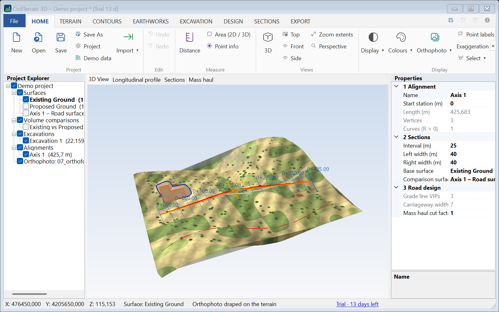
HOME → Orthophoto → Load orthophoto: choose a JPG, PNG, TIFF or GeoTIFF image. The georeference is read from the GeoTIFF tags or from the world file next to the image (.jgw, .pgw, .tfw, .wld) as exported by Pix4D, Agisoft Metashape, DJI Terra, QGIS and most CAD programs. The image must be in the project's coordinate system.
The orthophoto is draped on the surfaces (colour mode Orthophoto). Use Colours to return to elevation colours; the image stays in the project. Contours, axes and excavations are drawn on top of it. Large images are resized automatically up to 4096×4096 pixels for display.
8.3 A point cloud in its RGB colours as a gridded surface
Clouds from drones and photogrammetry (Pix4D, Agisoft Metashape, DJI Terra etc.) carry the colour (RGB) of every point. The program reads them as a gridded surface: one point per cell at the step you type and the average colour of the points in the cell. The surface is shown in the real colours of the site without an orthophoto and switches as usual between shaded, wireframe, shaded + wireframe or points (HOME → Display).
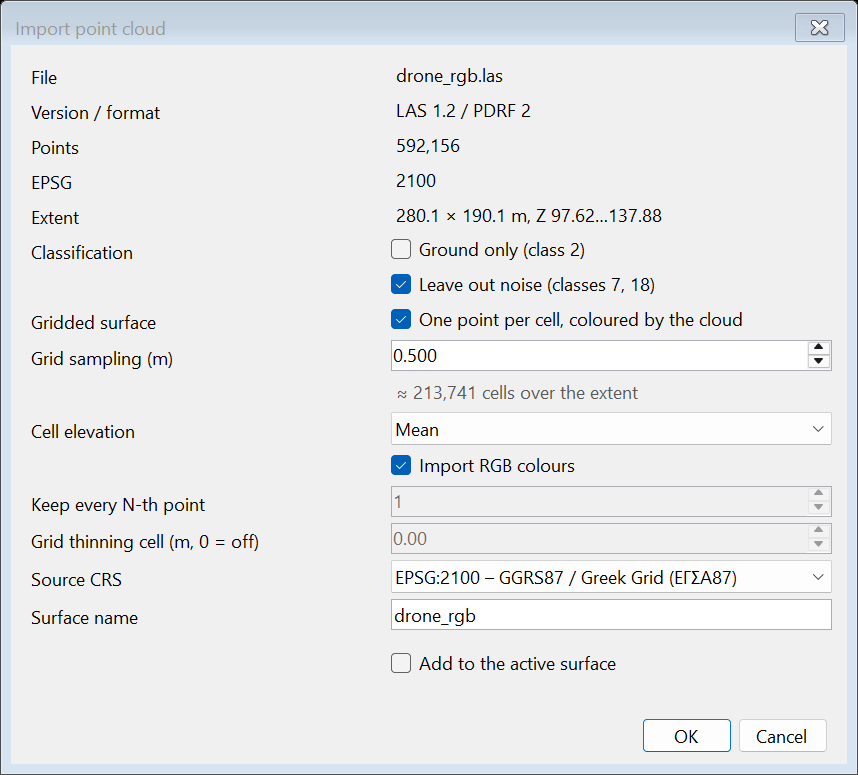
- HOME → Import → LAS / LAZ and choose the file.
- Tick Gridded surface (the default when the file has colours).
- Type the grid sampling in m. The program suggests a value close to the density of the cloud and shows how many cells it gives over the extent.
- Choose the cell elevation and whether the RGB colours are imported, and press OK.
| Option | Meaning |
|---|---|
| Grid sampling | Cell size (m). A smaller step gives more detail and a heavier surface: about 1 million cells are built in a few seconds; above 3 million a warning is shown. |
| Cell elevation | Lowest point (ground), mean or highest point (roofs, trees – the surface as the camera sees it). |
| Import RGB colours | The average colour of the points of every cell. 8- and 16-bit colours are recognised automatically (point formats 2, 3, 5, 7, 8, 10). |
| Ground only / leave out noise | Apply here too: e.g. the ground in its colours for a terrain model, or all classes for the picture of the site. |
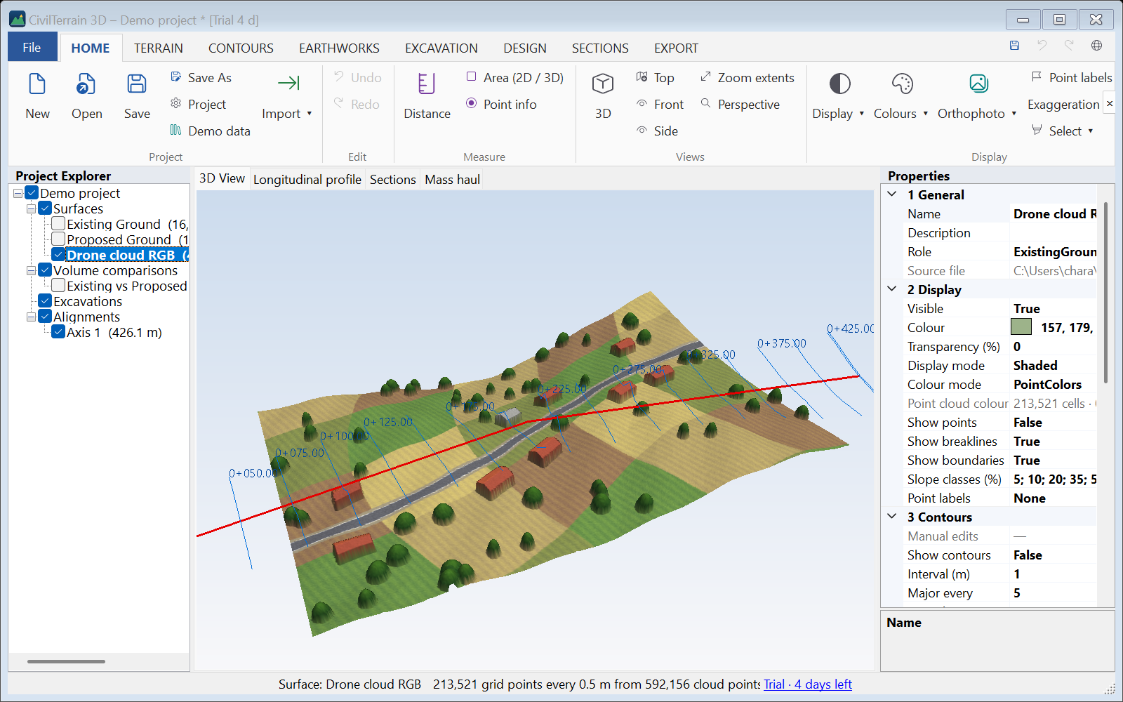
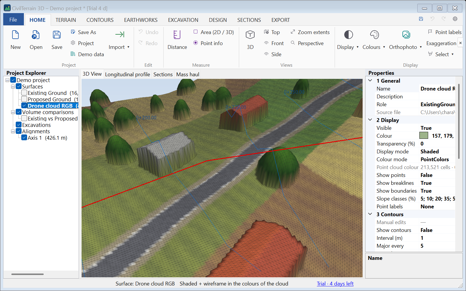
The new surface is coloured with Point cloud RGB (in the Properties: PointColors) and its contours are hidden at first. With HOME → Colours you switch to elevation colours, slopes etc. and back to the colours of the cloud at any time. The maximum triangle edge is set to 4 × the step, so that the gaps of the cloud (water, shadows) stay open instead of being bridged; change it in Surface data.
- The colours are saved in the project file and follow the surface when it is copied, smoothed or merged (where surfaces overlap, the first one has priority).
- With Add to the active surface the colours are added to the existing ones.
- If the source coordinate system differs from the project's, the colours are transformed together with the points.
Machines and trucks can be cleaned off such a surface too, together with their colours, with TERRAIN → Remove objects (section 10.4).
8.4 Following a road / channel
In a LiDAR or drone cloud the general ground filter (8.1) often cuts off the sharp edges of a road or a channel: the crest of the cut, the toe of the fill, the edges and the ditches. TERRAIN → Follow road / channel (the road-sign icon) solves this with the typical section:
- With the surface of the cloud active, draw a rough line along the road or channel, from its start. It does not need to be exact; it may be a few metres off. For Suggest points, draw it on the road (or in the channel): the two sides of the section are split at it.
- The dialog shows the first section (the points of the slice and their ground) with points suggested at the changes of slope. The suggested points stop at the crest and the toe, the outer ends of the steep faces (diamonds, free points); points on the natural ground beyond them are not suggested. A rough line at an angle to the road is allowed for. It is a proposal: check it, especially between walls or hedges, where it may put a crest on their top. Adjust the typical section: drag a point, double click to add one, right click to delete. Place the fixed points exactly on their edge (zoom with the wheel; the offset and Z show while you drag): they keep that distance along the whole road. In the table give the kind of each point (crest, toe, ditch, edge of pavement, axis, curb, channel lip / bottom…), which gives its name and code (TOP, TOE, DCH, SH, EP, AX, KR, CH, WALL; in the Greek interface ΦΡ, ΠΟ, ΤΑ, ΑΣ, ΑΞ, ΚΡ, ΡΕ, ΤΟ). For a channel, the suggested top of each side is a “Top of slope”; for a lined channel change its kind to “Channel – lip” (fixed). The crest and the toe are free points: they follow the ground however the height of the slope changes. The others keep the distances of the typical section and move together as one body, which may also tilt (superelevation).
- Follow: every few metres (e.g. 2 m) the program finds the typical section in the points, following the feature itself rather than the rough line. It ignores vehicles, vegetation and noise. It bridges gaps (e.g. no points under a bridge) and marks them as uncertain sections. The slider shows every section: green is the typical section found, blue the clean ground; the plan shows the lines.
- OK creates feature lines with their codes, optionally as breaklines of the surface so that the TIN keeps the edges. It also splits the points of the corridor into ground and objects (a disabled group), optionally with the general filter for the rest of the cloud (… and the general ground filter outside it), with the default settings of the ground filter and your last choice of Leave out low noise (section 8.1). Everything can be undone. The options of the result are in the strip Result (with OK): above the buttons and are always in view; the window fits whole also on a 1920 × 1080 screen at 150 % scaling.
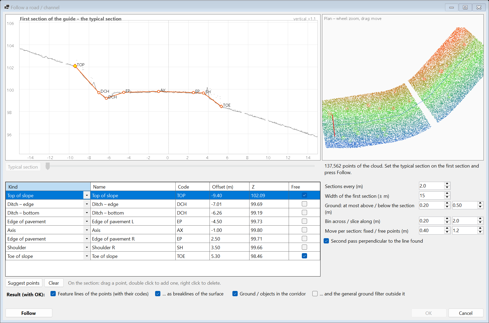
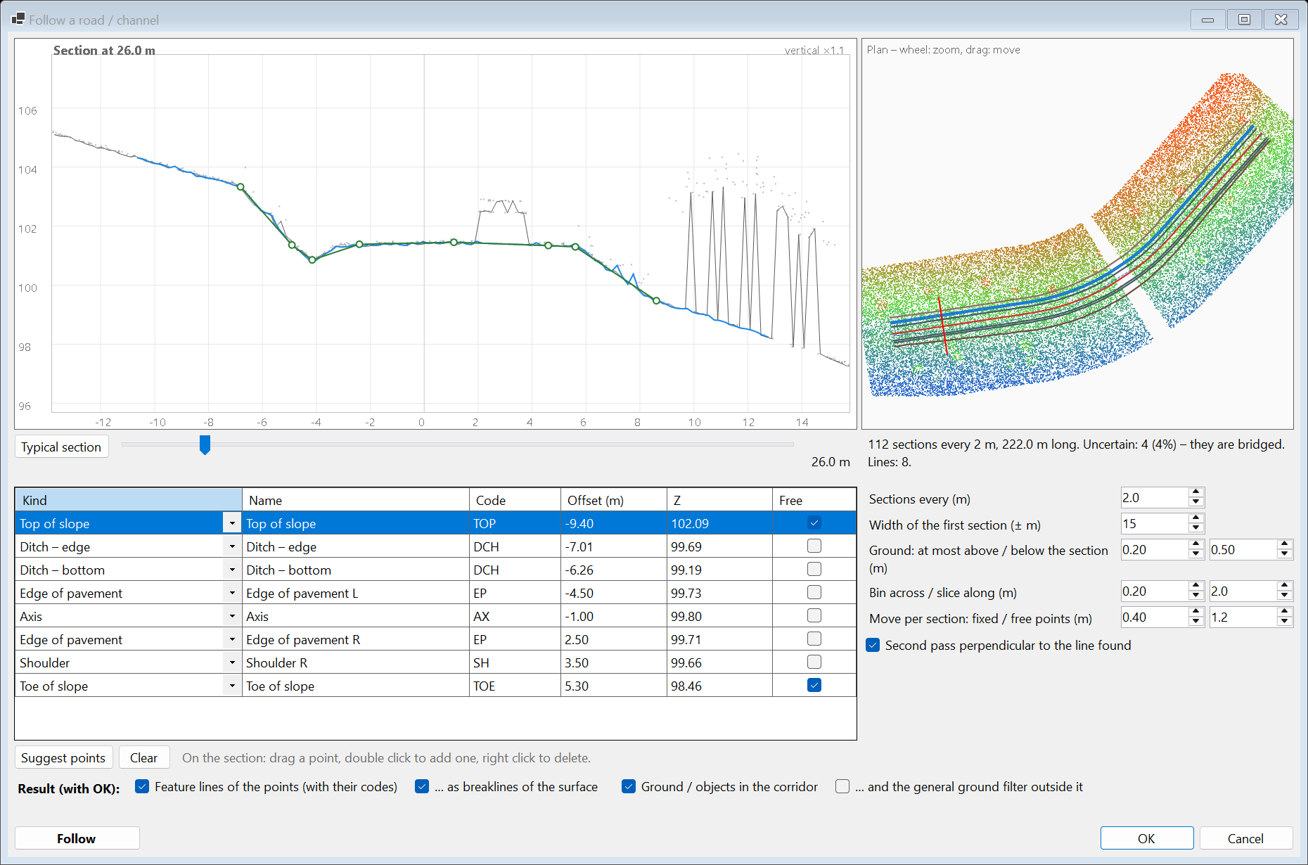
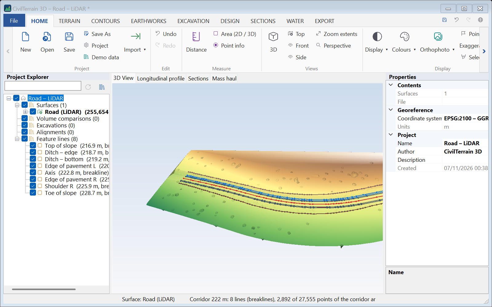
| Setting | Meaning |
|---|---|
| Sections every | Distance of the sections (1–5 m); smaller in tight curves. |
| Ground: at most above / below | How far above (e.g. 0.20 m) or below the ground of the section a point may be to count as ground. |
| Bin across / slice along | Resolution of the section (0.1–0.2 m) and length of the slice of points along it (2 m); make the slice longer in a sparse cloud. Suggest points reads a slice of at least 4 m (at most 6 m), straightened along the feature. |
| Move per section | How far the fixed and the free points may move from one section to the next. When the feature is lost the search widens by itself. |
Codes and DXF layers: the codes are in the language of the interface when the typical section is made, and they are never changed later (nor in older projects). In DESIGN → Drawing DXF / DWG every feature line goes on the layer FL_ + its code, in Latin letters: the English codes give e.g. FL_TOP, FL_TOE, FL_DCH, FL_SH, FL_EP, the Greek codes FL_FR, FL_PO, FL_TA, FL_AS. A project with typical sections made in both languages has two layers for the same kind of line (only FL_AX and FL_KR are shared).
12_dromos_lidar.las (a road with a cut, a ditch, a fill, vehicles and trees; an unclassified cloud, class 1, as it comes from the scan).9. Terrain model (TIN) and water flow
The TIN is built by Delaunay triangulation; breaklines and boundaries are inserted as mandatory edges (constrained Delaunay). The model is non-destructive: it keeps the source data and every edit and is rebuilt automatically after each change (TERRAIN → Rebuild TIN or F5).
9.1 Multiple surfaces
A project can hold any number of surfaces, e.g. Existing Ground, Proposed Ground, Excavation Surface, Final Construction Surface. Each has its own name, role, visibility, colour, transparency and contour settings.
9.2 Surface data – what takes part in the TIN
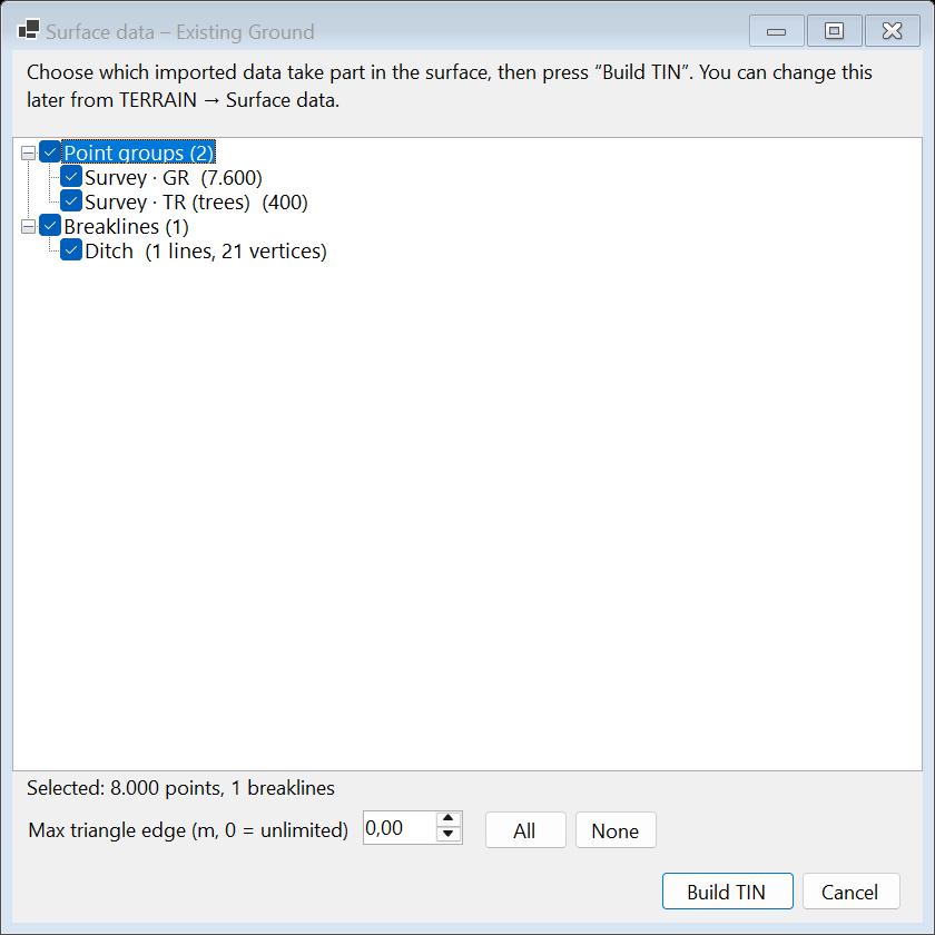
From TERRAIN → Surface data (or right-click the surface) you see all the data of the surface and tick which are used:
- Point groups – e.g. "Survey · GR" (ground), "Survey · TR" (trees). Untick groups that are not ground.
- Breaklines – grouped by name / layer / code.
- Boundaries – outer boundaries and holes.
- Max triangle edge length.
Click Build TIN. Changes can be undone. Disabled data are not deleted; you can enable them again at any time.
9.3 Surface simplification
Point clouds (LiDAR, drone) produce very large models. TERRAIN → Simplify reduces the points while keeping the maximum vertical difference you set (e.g. 0.05 m = 5 cm):
- only original points with their real elevations are kept;
- every original point is within the tolerance of the new surface;
- the outline, holes and breaklines are kept exactly;
- flat areas keep few large triangles, slope changes keep more.
A new surface is created (the original is kept hidden) and a summary is shown: points and triangles before/after, maximum and RMS difference, time.
9.4 TIN settings (Properties → 4 TIN)
| Setting | Description |
|---|---|
| Max edge length | Removes triangles with an edge longer than the value (cuts long "bridge" triangles at the edges). 0 = unlimited. |
| Duplicate tolerance | Points closer than the tolerance (default 1 mm) are treated as the same point. |
9.5 Statistics
TERRAIN → Statistics: number of points and triangles, plan and surface area, elevation range, mean slope, edge lengths, build time and any breaklines that could not be inserted.
9.6 Merging surfaces and point clouds
When an area is covered by several files (e.g. two drone flights, a LiDAR cloud with a supplementary GPS survey, an old and a new survey), TERRAIN → Merge surfaces (or right-click a surface → Merge with…) builds a new surface from the points, breaklines and boundaries of two or more surfaces. The original surfaces are not changed.
| Option | Description |
|---|---|
| Order of the surfaces | The order in the list (▲ ▼ buttons) is the priority: the first one wins where they overlap. |
| Common area | Only the points of the surface higher in the list are kept. Points of later surfaces that fall where it has data are left out. Its data means its triangles, without the long ones that only bridge empty space, such as the bay of an L-shaped survey. Their breaklines are cut exactly at the edge. Without this option all points are kept. |
| Height alignment | Every later surface is shifted vertically by the median difference from the first one in their common area (robust to vegetation and noise). The shift and its spread are reported at the end. |
| Grid thinning | One point per cell (nearest to the centre, lowest – for ground from a cloud – or mean). Breakline vertices are not thinned. |
| Longest triangle edge | For the new surface. The automatic value is the largest of the ticked surfaces; if one of them has no limit, the value is 0 (no limit). A mesh (LandXML, GeoTIFF etc.) counts with 1.5 × its longest edge. The value follows your selection until you type your own. |
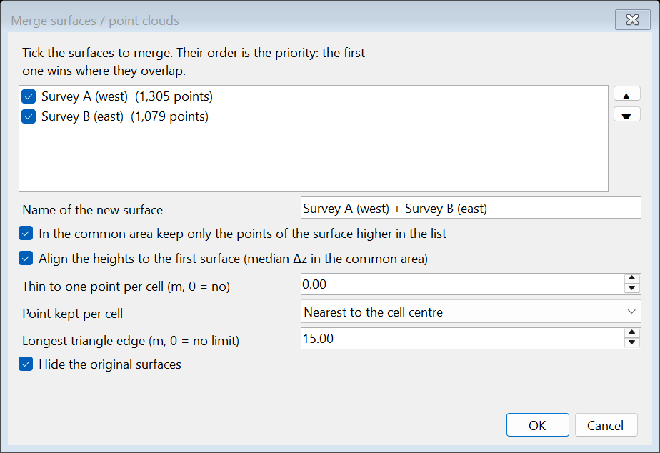
The points of every original surface become separate point groups with their numbers, so you can switch them on / off in Surface data. A mesh gives the vertices of its triangles.
Boundaries are handled as follows:
- Whatever a surface had cut away with its own boundaries (outer boundary, holes) stays out of the new one.
- Outer boundaries are kept only if every surface has one, so that none is cut away. A mesh counts with its outline.
- A hole hides only the data of its own surface. Where the other surfaces have data inside it, their data stays visible (show areas); if they cover it whole, the hole is left out. The report says so.
- The voids of a mesh (no data) become holes the same way, with the islands inside them as show areas.
At the end a report opens that shows for every surface:
- how many points were kept, cut away or left out in the overlap;
- the height shift.
The report stays open while you look at the new surface.
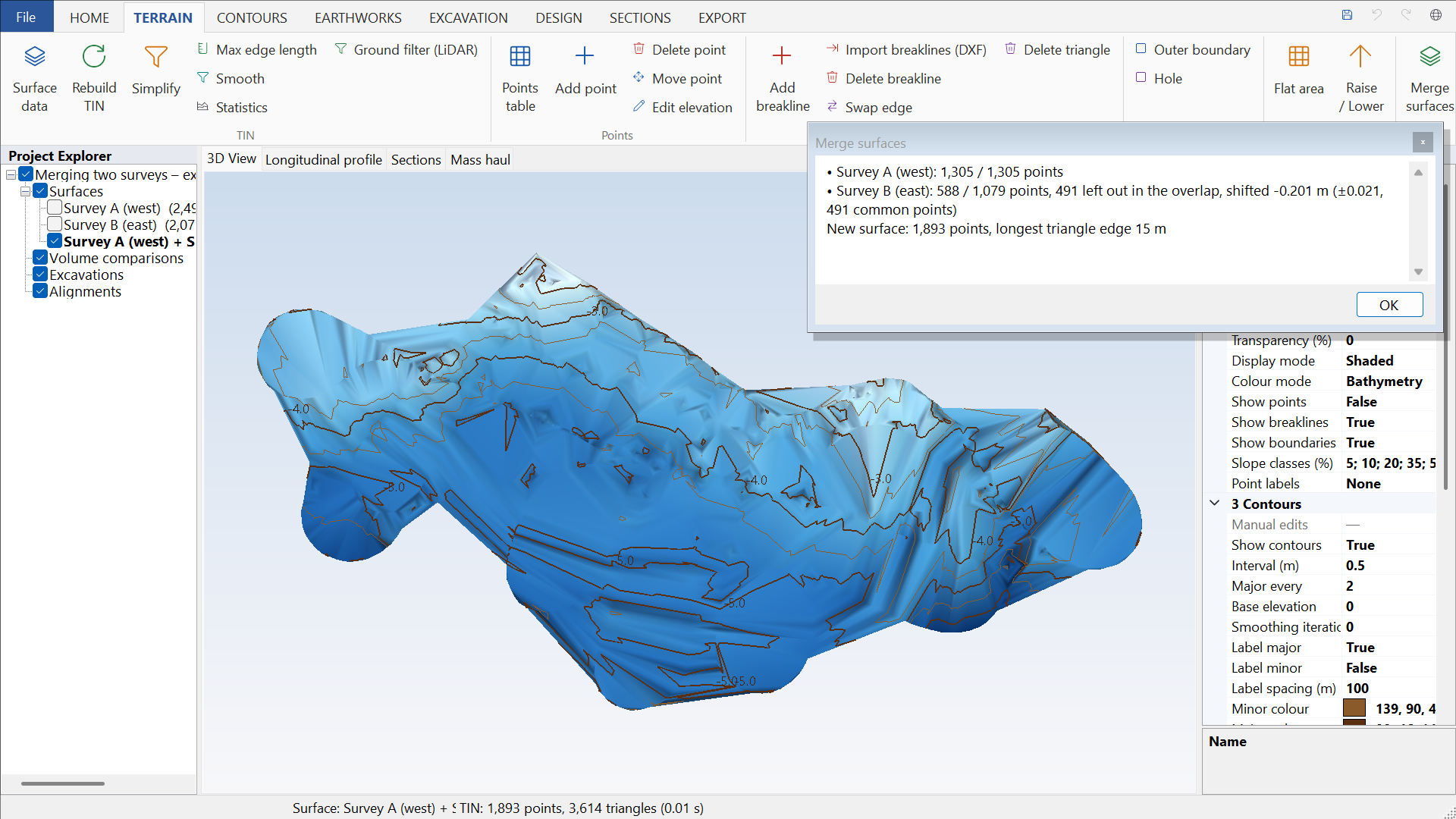
- If two surfaces do not touch, a longest triangle edge stops the gap between them from being bridged.
- A topographic survey that surrounds a lake or a river also “covers” the water with its triangles. For the bathymetry to count there, put the bathymetry first in the list or draw a hole in the topographic survey. The merge report points this out when points are left out far from the points of the earlier surface.
- To simply add a second file to an existing surface there is also Add to the active surface when importing.
9.7 Water on the surface: water courses and pools
WATER → Water on the surface: for the active surface the program shows where the rain water runs (water courses) and where it collects and stays (pools, with depth, area and volume of water). Use it to check a grading design before it is built, to find where manholes or culverts are needed, and to spot puddles on roads, squares and plots.
| Setting | Description |
|---|---|
| Grid spacing | The surface is sampled on a square grid. 0 = automatic (about 1.5 million cells, at a round spacing; the dialog shows the value). A finer grid shows smaller puddles and takes longer. |
| Water course from a drained area of | A line of the grid becomes a water course when its water comes from an area of at least this many m². The automatic value is about 0.5% of the surface. A smaller value gives more, smaller water courses. |
| Pools deeper than | Shallower pools are left out (e.g. 0.05 m). |
| Show the water courses / pools | What is drawn on the surface. |
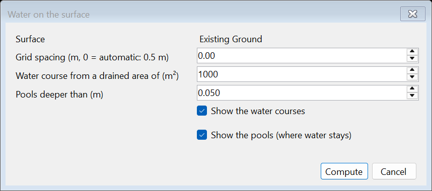
The water courses are drawn in blue, reach by reach from junction to junction, thicker and darker the larger their basin. Where the ground falls towards the edge of the surface, the water leaves there and does not run along the edge. Through the holes of the surface (hidden areas, deleted triangles, e.g. the opening of a culvert under a road) the water passes at the level of their edge: it is neither lost in them nor dammed by them, at whatever angle they lie. The pools are coloured blue, darker where the water is deeper, up to their spill level, that is up to where the water rises before it overflows. A list of the pools also opens, largest first. For each pool it shows the lowest point, the depth, the area and the volume of water. Clicking a row zooms to the pool in the drawing. Clicking a header sorts the column. WATER → Pools opens the list again.
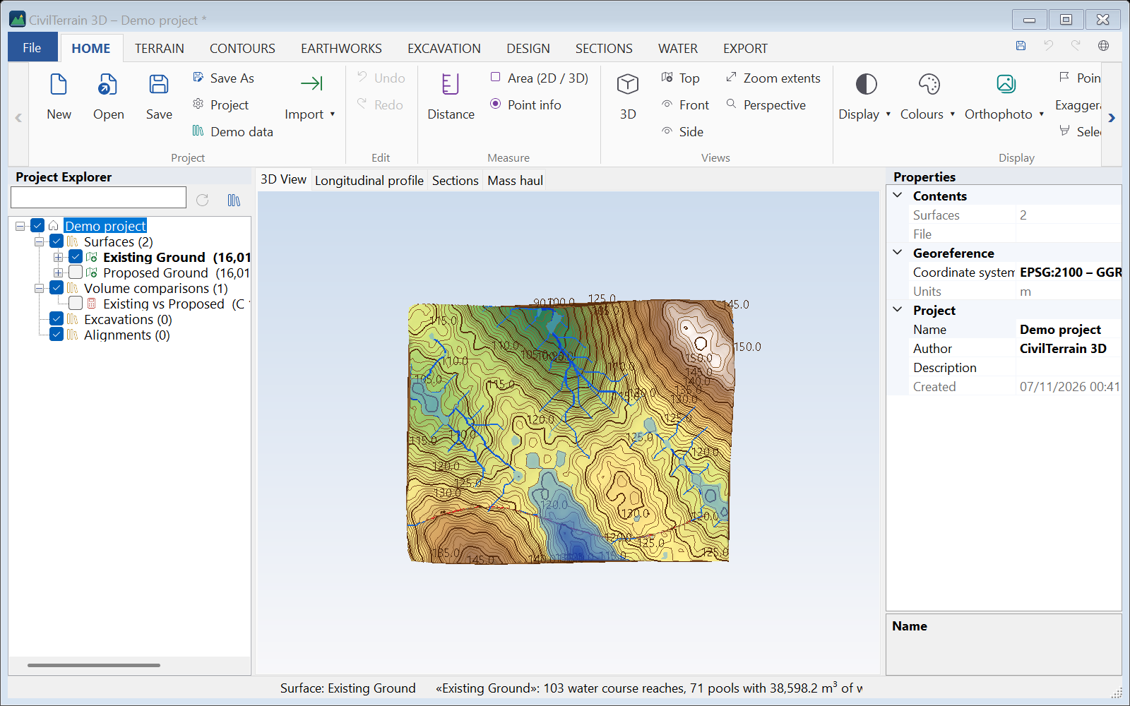
The computation runs in the background and Esc cancels it. The water picture goes with Hide the water, when the surface changes or when another project opens. It is not saved in the project: run the command again whenever you need it.
9.8 Drainage basin
WATER → Drainage basin: click the point where the water leaves (culvert, manhole, lower end of a water course). The program finds the whole area upstream, from where the water ends up there, and adds it to the project tree as a drainage basin. The click snaps to the water course with the largest basin within a short distance, so it does not need to be exact. A click inside a hole of the surface (e.g. on a hidden culvert) takes as outlet the point where the water leaves the hole.
For each basin the program computes:
- the area (m², ha, km²), the perimeter and the outline;
- the longest flow path L, from the farthest point to the outlet, and its grade;
- the outlet elevation, the mean and the highest elevation, and the mean grade of the ground;
- the time of concentration by Kirpich (tc = 0.0195 · L0.77 · S−0.385 min, with L in m) and by Giandotti (tc = (4√A + 1.5 L) / (0.8 √(Hm − H0)) hours, with A in km² and L in km);
- the peak flow by the rational method, Q = C · i · A / 3.6 (m³/s, with i in mm/h and A in km²). You give the runoff coefficient C and the rainfall intensity i in the Properties; the peak flow updates at once.
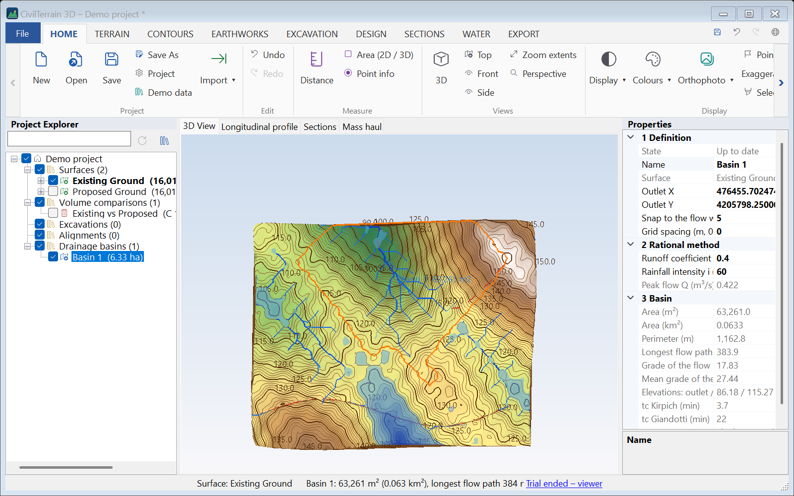
In the Properties you can also change the outlet (X, Y), the snap distance and the grid spacing. After such a change, or when the surface changes, the basin shows as out of date (⚠) until you Recalculate it (right-click the basin). The right-click menu, and the buttons of the Drainage basins group for the selected basin, also have Results… and the export to Excel and DXF / DWG. The DXF has the outline on the ground (layer BASIN), the longest flow path (FLOW_PATH), the outlet (OUTLET) and, if the water courses are shown, their reaches inside the basin (STREAMS). Basins are saved in the project and computed again when you open it.
10. Terrain editing
The TERRAIN tools act on the active surface. Every edit supports Undo (Ctrl+Z) and Redo (Ctrl+Y).
10.1 Drawing on screen
- Click = vertex. The cursor snaps to TIN vertices.
- Enter, double-click or right-click = finish the line/polygon.
- Backspace = remove the last vertex, Esc = cancel.
- Each tool's prompt is shown in the status bar.
The Add / Delete point, Edit elevation, Delete breakline, Swap edge and Delete triangle tools stay active after each click so you can edit many items in a row. Press Esc to finish.
10.2 Tools
| Tool | Usage |
|---|---|
| Add point | Click the position and type the elevation (the surface elevation is suggested). |
| Delete point | Click on the point (or a breakline vertex). |
| Move point | Click the point, then click the new position (elevation is kept). |
| Edit elevation | Click the point and enter the new Z. |
| Add breakline | Draw a polyline; elevations are taken from the surface (or asked outside it). |
| Delete breakline | Click near the line. |
| Import breaklines (DXF) | Adds the polylines of the selected layers as breaklines to the active surface. |
| Swap edge | Click an edge: flips the diagonal of the quadrilateral (only if convex). |
| Delete triangle | Click inside the triangle. |
| Outer boundary | Closed polygon: everything outside is removed. The boundary is inserted exactly into the TIN. |
| Hole | Closed polygon: everything inside is removed (e.g. buildings, ponds). |
| Flat area | Closed polygon and elevation: creates a level pad. |
| Elevation offset | Δz on the whole surface or inside an outline, with a transition band, in place or into a copy (section 10.3). |
| Remove objects | Machines, trucks and other objects off the ground, found automatically or drawn; the ground under them is made from the ground around them (section 10.4). |
| Replace terrain | Debris or a deposit inside an outline comes down to the ground around it (section 10.5). |
| Smooth | Creates a new smoothed surface; the original is preserved. Breaklines and boundaries are kept fixed. |
| Duplicate / Delete | Copies or deletes the active surface. |
10.3 Elevation offset
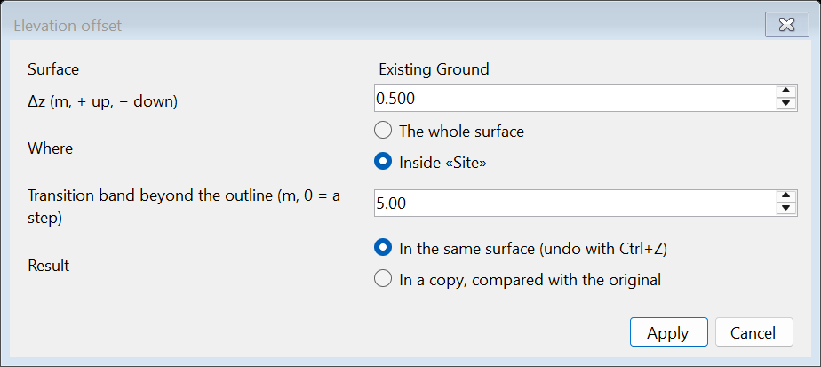
TERRAIN → Elevation offset: moves the elevations of the active surface by Δz (positive: up, negative: down).
| Setting | Description |
|---|---|
| Where | On the whole surface or inside an outline. If a zone, a closed line or an outline (of polygon earthworks, a grading optimization, a sloped design) is selected in the tree, that one is used; otherwise you draw it after OK. |
| Transition band | Beyond the outline the offset fades smoothly to zero over this distance, so that no step forms. 0 = an abrupt change right at the edge. On point surfaces, points are added along the outline and the band, so that the change follows the outline also where the survey points are sparse. Breaklines that cross the outline or the band get vertices there and follow too. |
| Result | In the same surface (undo with Ctrl+Z), or into a copy: the original is hidden and a volume comparison original → copy is made. |
10.4 Remove objects
A drone or LiDAR survey of a site often keeps machines, trucks, cars or containers. The surface rises over them, and volumes, contours and cross sections count them as ground. TERRAIN → Modify → Remove objects takes them away: inside each outline the ground is made again from the ground around it. It works on point clouds, gridded RGB clouds (section 8.3) and DEM / DSM.
- Make the surface active. To search only part of it, or to use an outline that already exists, select that outline in the tree: a zone, a closed line, the outline of polygon earthworks, a grading optimization, a sloped design, a building-code check, a section grid or a spot grid, a closed breakline or a boundary.
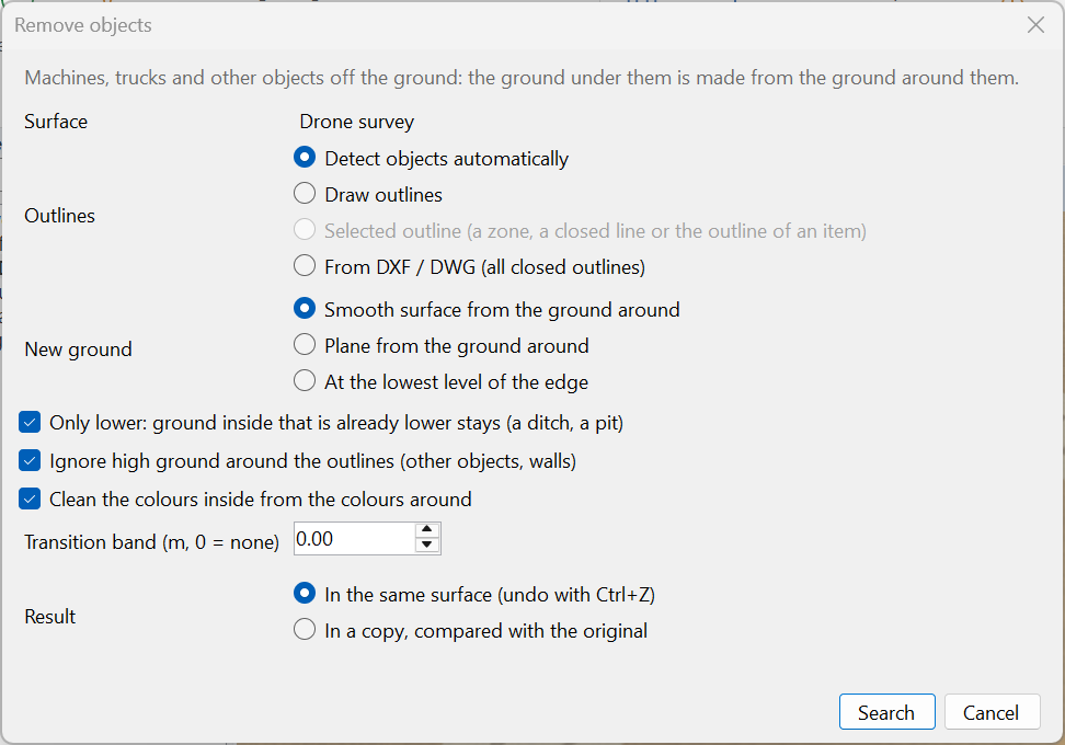
- TERRAIN → Modify → Remove objects. In the window choose where the outlines come from, how the new ground is made and where the result goes. The button follows the source: Search, Draw, Open… (DXF / DWG) or Apply (selected outline).
- Check the list of the objects found, or draw the outlines, and press Apply.
| Setting | Description |
|---|---|
| Outlines | Detect objects automatically (default): the program finds the objects and lists them for you to check. With an outline selected in the tree, Search only inside «…» keeps the objects whose centre is inside it. Draw outlines: draw as many as you like, one after the other. Selected outline «…»: applied at once. With nothing selected it reads Selected outline (a zone, a closed line or the outline of an item) and cannot be chosen. From DXF / DWG (all closed outlines) of the layers you choose: they are shown in the view and you can draw more before applying. |
| New ground | Smooth surface from the ground around (default): carries on the slopes of the ground around the outline smoothly; a sloping plane comes back exactly. Plane from the ground around: for each outline the plane that fits the ground around it best, without the values that stand out above it. At the lowest level of the edge: level, for each outline at the low ground around it (about its lowest 5%). Outlines that touch or overlap share one plane or level; outlines that only lie close (a deposit on the floor and one on the bench above it) each stand on their own ground. |
| Only lower | Ticked by default: the surface only comes down, and ground inside that is already lower than the new ground (a ditch, a pit) stays as it is. Without it, lower points are raised to the new ground too. |
| Ignore high ground around the outlines | Ticked by default for Remove objects. Ground around the outline that is much higher than the low ground next to it (more than about 0.30 m: another truck touching it, a wall) is not used, so it does not lift the new ground. The program says what share was ignored. |
| Clean the colours inside from the colours around | For surfaces with colours (a gridded RGB cloud): the colours of the ground around replace those of the machine. Disabled when the surface has no colours. An orthophoto, if any, does not change. |
| Transition band (m, 0 = none) | Beyond the outline the new ground joins the old one smoothly over this distance. 0 (default) = the change is right at the outline. |
| Result | In the same surface (undo with Ctrl+Z), the default: all the outlines in one edit. In a copy, compared with the original: a surface “… (objects removed)” is made, the original is hidden and a volume comparison original → copy is added, whose cut is the volume taken away. |
The choices are kept, separately for each command, until the program closes.
Automatic detection and the review list
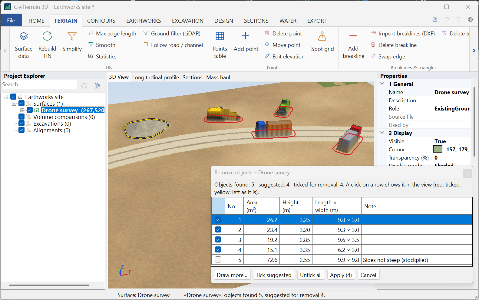
With Search the program searches in the background (Esc cancels) for objects standing on the ground: at least 0.80 m higher than the ground around them, with a plan area of about 3 – 150 m² and up to 15 m long (up to 22.5 m for wide and high machines, e.g. an articulated dump truck). For each object it proposes an outline 0.75 m outside it. The list Remove objects – … with the name of the surface then opens at the bottom right inside the view, as large as its rows (at most 40% of the height of the view):
- The suggested objects are already ticked: they have the size and plan of a machine, steep sides, a flat top and lower, even ground all around them.
- The others are not ticked, and the Note column says why, e.g. “Sides not steep (stockpile?)”, “No flat top (stockpile, tree?)”, “Ground not lower all around (cut face, crest, edge?)”, “Long and narrow (berm, windrow?)” or “Smaller than 3 m²”. So stockpiles, berms and cut faces are not removed by mistake.
- Columns: No, Area (m²), Height (m) (of the body above the ground around it: a raised boom or mast does not count), Length × width (m), Note; a click on a header sorts. A click on a row shows the object in the view and zooms to it; a click on its check box or Space changes the tick. In the view the ticked ones are red and those left as they are yellow.
- Tick suggested and Untick all change all the ticks at once.
- Draw more…: draw outlines for anything not found. They go into the list ticked, with the note “Drawn”. In the small drawing window, Back to the list or Esc takes you back to the list; the outline being drawn goes into it if it has three vertices or more (Esc with one or two vertices starts it again). If another tool takes the view meanwhile, the drawing ends and the list stays; an outline cut short (three vertices or more) goes into the list unticked, with the note “Drawn, cut short by another tool: tick it to remove it”.
- Apply (N) removes the N ticked objects in one edit; Cancel closes the list without changes.
If no object is found, the program asks whether you want to draw their outlines.
Drawing several outlines
With Draw (or after the DXF / DWG) you draw the outlines one after the other. A small window at the top right of the view shows how many outlines you have and how many vertices the current one has:
| Key / button | Action |
|---|---|
| Click | A vertex. A click on a vertex or a side of another outline snaps to it (shared edges with no gaps). |
| Enter / double click | Outline done; the next one starts by itself. |
| Backspace / Back | Back one vertex. |
| Undo outline | Takes away the last outline. |
| Apply (N) | Applies all the outlines in one edit, and the current one if it has at least three vertices. |
| Esc / Stop | Ends the drawing. If there are outlines, the program asks: Yes = apply, No = discard, Cancel = go on drawing. The current outline counts if it has at least three vertices. Esc while the current outline has one or two vertices only starts that outline again. |
An outline with one or two vertices is drawn again; an outline whose sides cross is not added. While a surface is being rebuilt, Apply is refused: the drawing goes on and you press Apply again when it is done.
If another tool takes the view while you draw (a measurement, another command), nothing drawn is lost: the drawing waits with its outlines in the view, the current outline is kept if it has three vertices or more, and the small window says “Paused: another tool has the view.” Continue drawing (in place of Back) goes on with the drawing; Undo outline, Apply (N) and Stop work as before. If nothing had been drawn, the command ends.
The result
The status bar says what was done, the volume first, e.g. “Remove objects: removed 110.3 m³, outlines 1, area 68 m², points changed 147, colour cells cleaned 147”; “added … m³” follows the removed volume when it is at least 0.05 m³, and into a copy the line ends with the name of the copy. The volumes are measured on the surface itself, between the surface before and after, so into a copy they are the cut and fill of the comparison. What changes for each kind of surface:
- Point cloud: the elevations of the points inside the outlines (loose points and enabled groups; disabled groups, e.g. the “objects” of the ground filter, do not change). Enabled breaklines that cross the outlines get vertices and follow the new ground. On a sparse survey, with few points inside an outline, points of the new ground are added in a new point group “Remove objects”.
- Gridded RGB cloud (section 8.3): as a point cloud, and the colours are cleaned too, so that ground shows where the machine was.
- DEM / DSM and other fixed meshes (GeoTIFF, LandXML, OBJ, PLY): only the elevations of the vertices change; the triangles stay the same and the surface stays a mesh. The status bar says “vertices changed”.
When only elevations change, the TIN is updated without a new triangulation, and the result comes in a few seconds even on millions of points. In the same surface, one Ctrl+Z undoes all the outlines together. Anything computed from the surface (comparisons, spot grids etc.) is updated. If nothing changed (e.g. the outlines are off the surface, or with “Only lower” the ground inside is nowhere higher than the new ground), the program says so and why, with no undo step and no copy.
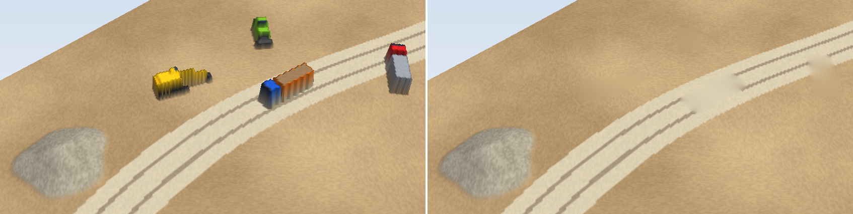
After applying, warnings may be shown:
| Message | What it means |
|---|---|
| “…% of the area inside the outlines is not on the surface: it is left as it is.” | The outline goes off the survey; only its part on the survey changes. |
| “… part(s) of the area have no ground around them on the surface and were left as they were.” | There is no ground around to give elevations (e.g. the outline covers the whole surface). Make the outline smaller. |
| “…% of the ground around the outlines is much higher than the ground next to it (another object, a wall) and was not used.” | The effect of “Ignore high ground”. If the share is large and there is a bank next to the outline, see the limits below. |
| “The colours were not cleaned: the outlines cover too many colour cells (…).” | More than 3 million colour cells; the elevations changed as usual. Apply to smaller outlines. |
| “The outlines are outside the surface: nothing was changed.” | Check the active surface and the coordinate system of the DXF. |
- The automatic detection is tuned for machines and vehicles on open ground. Check the list before applying: a tree with a steep crown may be suggested, and an object of an unusual shape may not be.
- A machine against a wall or a cut face is not suggested (“Ground not lower all around…”): tick it in the list or draw its outline. Objects that touch each other are found as one; if together they are longer than 22.5 m they are not suggested (“Longer than …”), and a truck with a trailer may come out “Long and narrow”. Draw their outlines then.
- With “Ignore high ground”, a sharp bank, kerb or step right next to the outline is taken for an object too, and the new ground comes out lower. Draw the outline a little away from the bank, or untick the option.
- The new ground is an estimate from the ground around: it does not “know” what lies under a large object. On large outlines the computation spacing grows by itself (e.g. about 0.4 m on a 9 ha outline), so the new ground is coarser there; the volumes are still measured on the surface itself.
10.5 Replace terrain
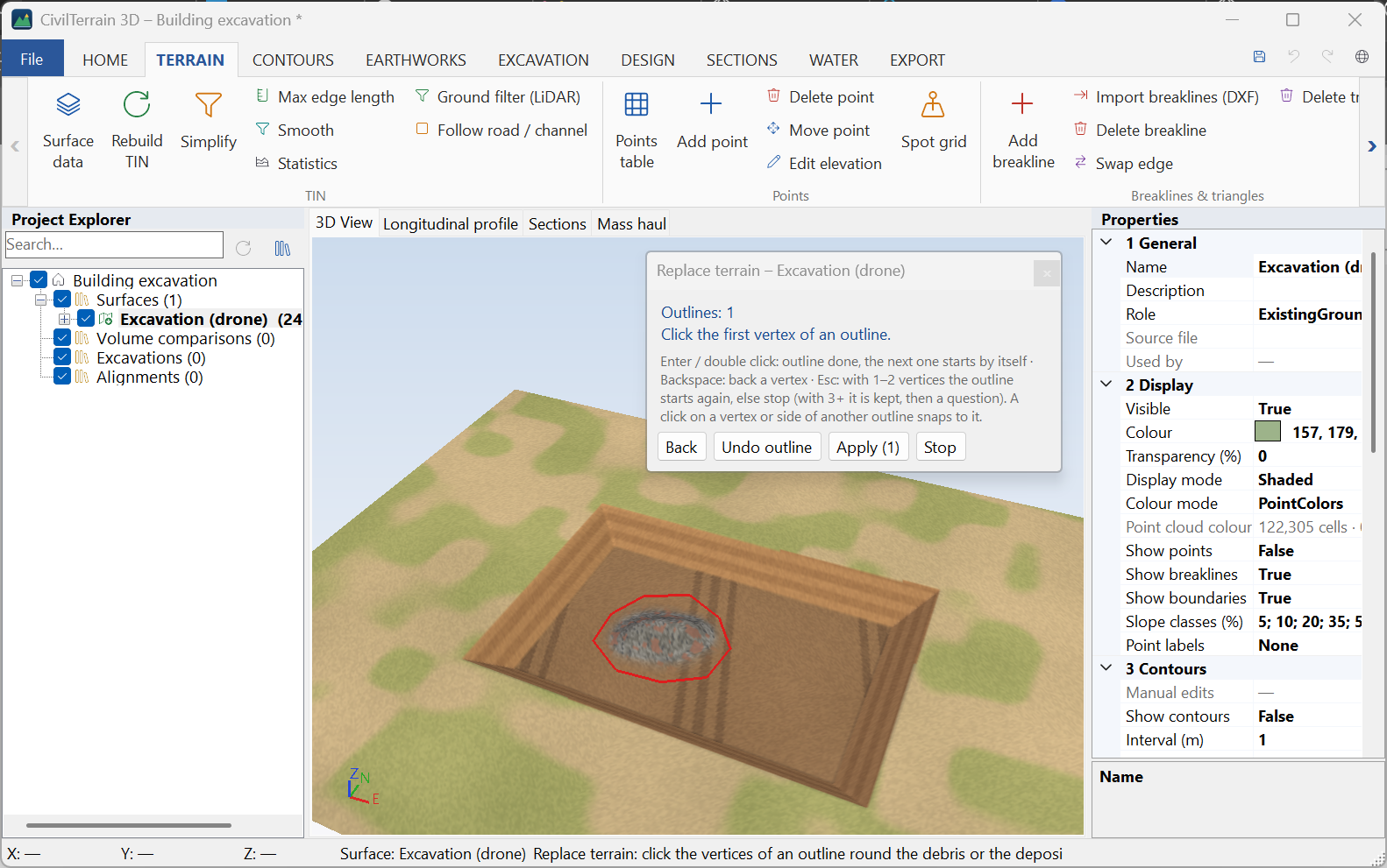
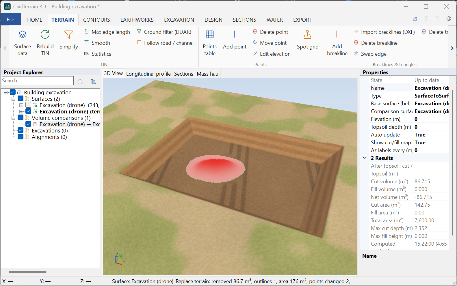
Inside an excavation or on a platform there is often debris, a pile or a deposit of material that is not part of the ground you want to measure. With TERRAIN → Modify → Replace terrain you encircle it, and the ground inside the outline comes down to the ground around it (smoothing).
The window is the same as for Remove objects (section 10.4), without the automatic detection, and with two other defaults:
- the outlines are drawn (or come from the selected outline or a DXF / DWG);
- Ignore high ground around the outlines is not ticked: banks, benches and berms crossing the outline are ground and are used, so the new ground is not pulled down.
The Smooth surface carries on the banks and slopes around; At the lowest level of the edge gives a level floor, e.g. for material on the bottom of an excavation. With Only lower (default) lower points inside the outline (pits, ditches) stay as they are. The new ground takes its elevations from a strip about 1 m outside the outline: draw it so that it runs over clean ground.
You draw as many outlines as you like with the same small window (Back, Undo outline, Apply (N), Stop) and they are applied together, with one undo. In a copy, the new surface is named “… (terrain replaced)”.
11. Contours
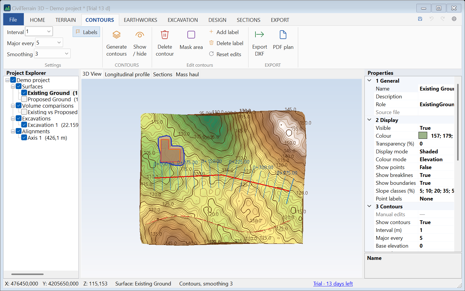
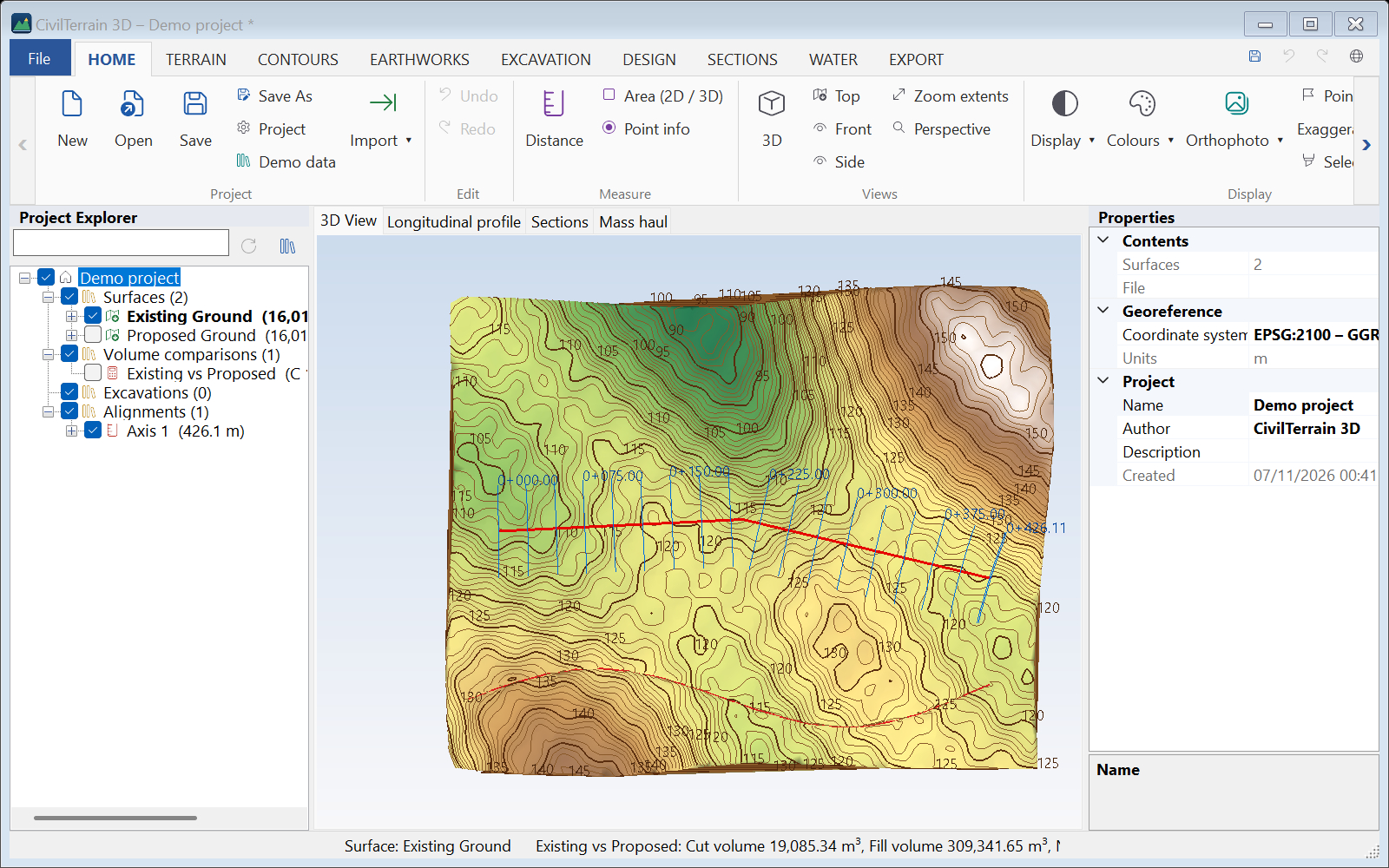
Contours are computed exactly from the TIN and shown in 2D and 3D. On the CONTOURS tab set:
| Setting | Description |
|---|---|
| Interval | Contour interval (e.g. 0.5 – 1 – 2 m). Type and press Enter. |
| Major every | Every how many contours a major (thicker) contour is drawn. |
| Smoothing | 0 = exact TIN lines, 1–6 = progressively smoother curves. End points at the boundary do not move. |
| Labels | Switches the elevation labels on / off; Labels… sets which contours and every how many metres (below). |
Changes apply immediately to the active surface. Colours, base elevation and labels are also in Properties → 3 Contours.
Export: Export DXF (layers CONT_MAJOR, CONT_MINOR, CONT_LABELS with the elevation on every polyline) and PDF plan.
Contour labels
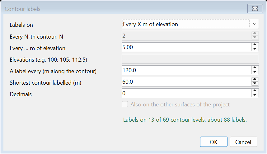
CONTOURS → Labels… sets which contours get elevation labels and every how many metres:
| Setting | Description |
|---|---|
| Labels on | Major, minor, all contours, every N-th contour, every X m of elevation (e.g. every 5 m: 100, 105, 110… whatever the interval) or given elevations you type (e.g. 100; 105; 112.5). |
| A label every | Distance of the labels along the contour (m). |
| Shortest contour labelled | Shorter contours (e.g. small closed islands) get no label. |
| Decimals | 0–3 decimals in the text. |
The dialog shows at once how many levels and about how many labels you get. Also on the other surfaces applies the settings to all of them. The labels are used on screen, in DXF / DWG, PDF and the drawing sheets. The Labels button switches them on and off without losing the settings. The same settings are also under Properties → 3 Contours.
11.1 Editing contours
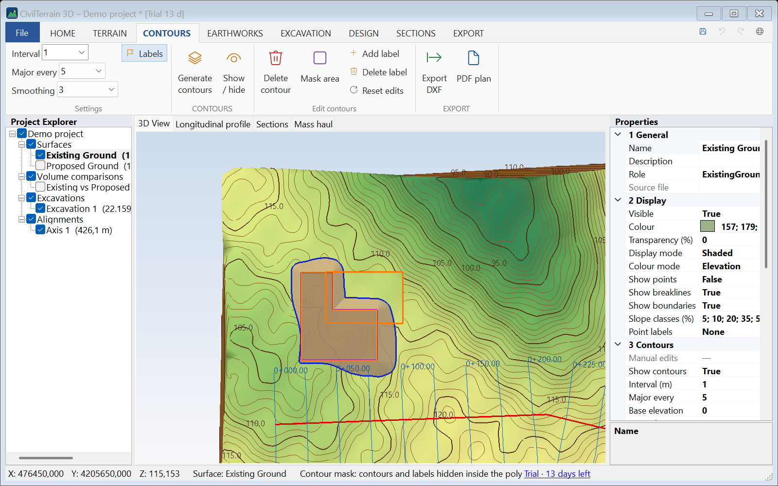
The CONTOURS → Edit contours group improves the drawings without changing the terrain. The edits are stored in the project, apply to DXF/PDF exports and can be undone with Ctrl+Z:
| Tool | Use |
|---|---|
| Delete contour | Click a contour: that piece is removed (e.g. small "islands"). Repeating, Esc to finish. |
| Mask area | Polygon inside which contours and labels are hidden (buildings, roads, squares). |
| Add label | Click a contour: an elevation label is added there, aligned with the line. |
| Delete label | Click a label to remove it. |
| Reset edits | Removes all manual edits of the active surface. |
12. Earthwork volumes
12.1 Comparing two surfaces
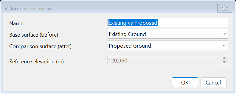
- EARTHWORKS → Volume comparison.
- Choose the base surface (before) and the comparison surface (after). Examples: Existing → Proposed, Existing → Excavation, Before → After.
- Results appear in Properties and in the status bar.
For surface vs elevation (e.g. a stockpile above a level) use Surface vs elevation.
12.2 Results
| Quantity | Meaning |
|---|---|
| Cut volume | Where the comparison surface is below the base (m³). |
| Fill volume | Where the comparison surface is above the base (m³). |
| Net volume | Fill − cut (positive = excess fill). |
| Cut / fill / total area | Plan areas (m²) – only the common valid area of both surfaces. |
| Max cut depth / fill height | Maximum elevation difference in cut and fill. |
| Centroids | In the Properties, category 3 Centroids: Cut centroid X / Y / Z, Fill centroid X / Y / Z and the horizontal distance between them (Centroid distance). Z is the mean elevation of the volume. With topsoil, also the centroids after stripping it. See “Centroids of the volumes” in section 12.6. |
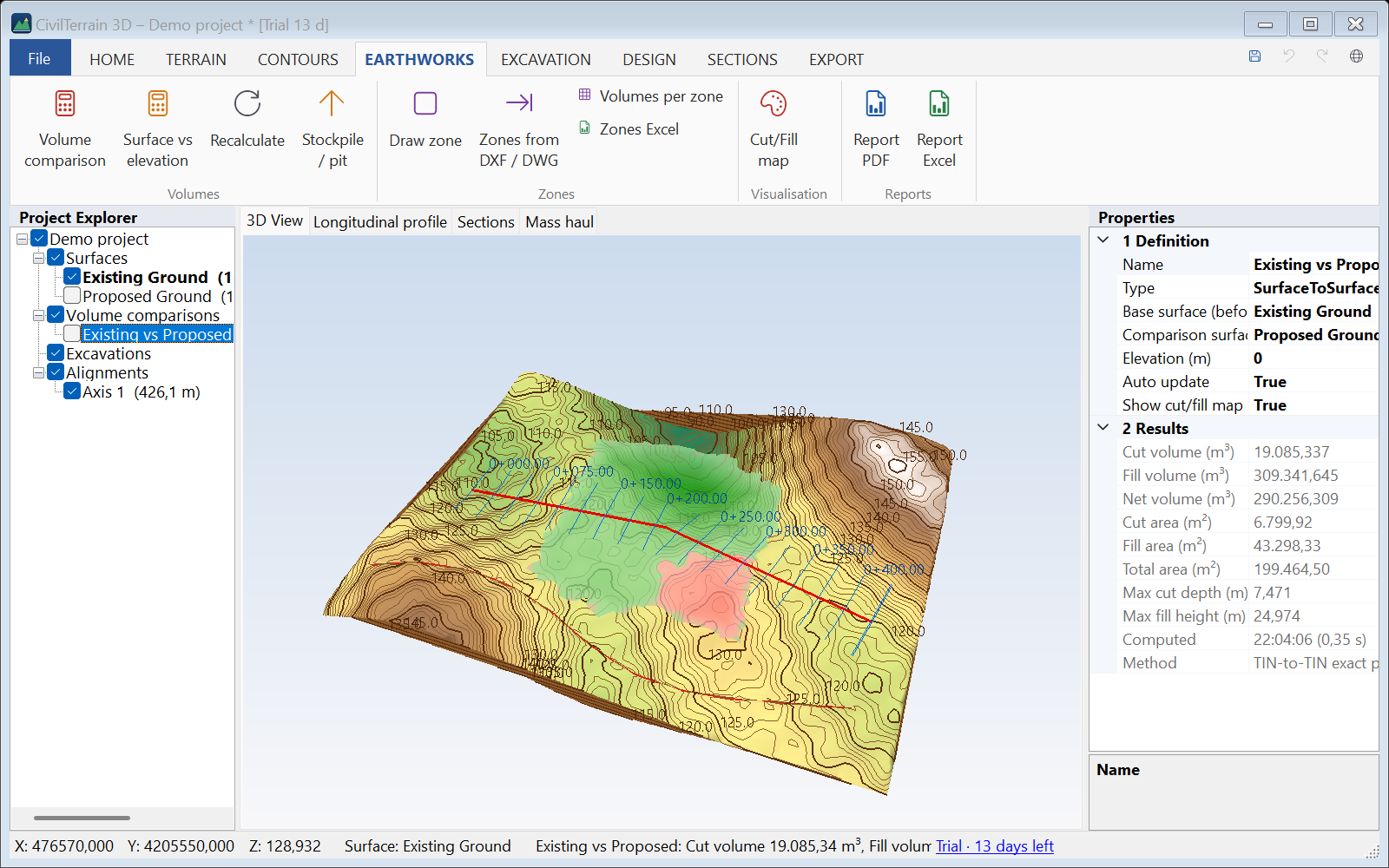
The cut/fill map is toggled with its button or the tree check box: red = cut, green = fill, intensity shows the depth.
12.3 Stockpile or pit volume
EARTHWORKS → Stockpile / pit: draw the toe of the stockpile (or the rim of the pit) on the surface. Choose the base:
| Base | When |
|---|---|
| Triangulated from the outline | The most common: the base follows the ground at the toe (stockpiles on sloping ground). |
| Best-fit plane | Least-squares plane through the outline points. |
| Lowest / mean elevation | Horizontal base at the lowest or mean outline elevation. |
| At elevation… | Horizontal base at a given elevation. |
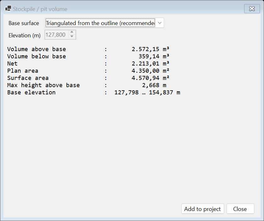
The dialog shows volume above/below the base, net volume, 2D/3D areas and maximum height. If part of the outline is off the surface, its shape is kept and the share that does not count is shown. Add to project creates the base surface and a ground → base comparison for PDF/Excel reports: cut = material above the base (stockpile), fill = the pit below it.
12.4 Volumes per zone
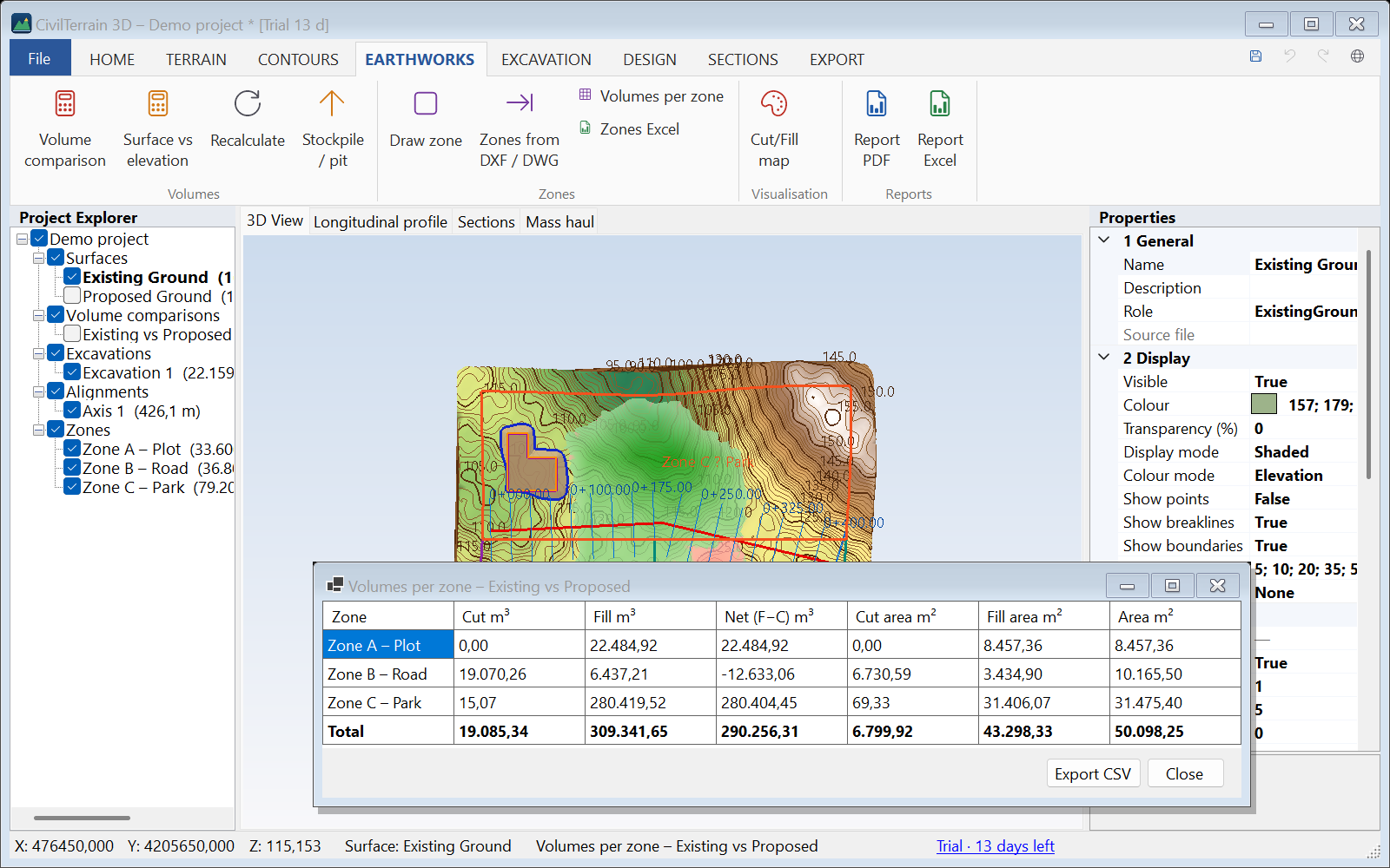
To split volumes into parts (plots, phases, contracts): EARTHWORKS → Draw zone and give a name. Zones are drawn on the plan and listed in the project tree (rename / delete with a right click).
Volumes per zone gives, for the selected comparison, cut, fill, net volume and areas exactly for each zone (the computation pieces are clipped at the zone boundary). If no comparison is selected and there are several, the program asks which one. The % outside column shows the part of a zone without both surfaces, and overlapping zones are warned about (they count twice in the totals). With topsoil in the comparison a topsoil column is added. Zones are included automatically in the PDF (all of them, over as many pages as needed, and drawn on the plan) and Excel reports.
12.5 Volume zones from DXF / DWG
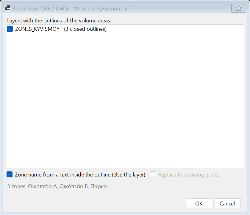
When the outlines of the volume areas already exist in a CAD drawing, there is no need to draw them: EARTHWORKS → Zones from DXF / DWG.
- Choose the layer(s) with the closed outlines; a polyline whose first and last vertex coincide also counts as closed. Arcs and circles become polygons.
- The name of each zone comes from a text (TEXT/MTEXT) inside the outline — the smallest outline containing it, for nested areas — otherwise from the layer name.
- Replace the existing zones or add to them; the import can be undone with Ctrl+Z.
- If a computed volume comparison exists, the volumes-per-zone table is offered right away; zones are also included in the PDF/Excel reports.
Sample: 10_zones_kyvismou.dxf.
12.6 Polygon earthworks (plot, pad)
The most common question: "how many cubic metres to grade this plot to +102.50, at 2 %, or balanced?". EARTHWORKS → Polygon earthworks answers it in one step, without building surfaces and comparisons.
Choosing the polygon
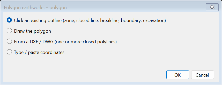
- If a zone or a closed feature line is selected in the tree, it is used straight away (also with right click → Polygon earthworks…).
- Otherwise choose: click an existing outline (zone, closed feature line, closed breakline, surface boundary, excavation outline or daylight — a click inside a zone is enough), draw, from DXF / DWG (one or more closed polylines, named from the text inside) or type / paste coordinates (e.g. from Excel or the survey).
Design
| Graded to | What is computed |
|---|---|
| Horizontal level | Cut / fill to elevation Z. Lowest / Mean / Highest ground give a starting value, and the slider changes Z with instant results. |
| Inclined plane | Plane with a grade % falling towards an azimuth (grads, clockwise from north) through the reference point at elevation Z. It can also be set From 3 points… (clicks on the surface) or as the Best-fit plane of the ground inside the polygon (least squares). |
| Other surface | Ground versus a design surface (or a later survey) inside the polygon only. |
| Depth below the ground | Uniform excavation, e.g. 0.50 m (stripping, sub-base). |
Elevation: "Elevation I give", Balance cut = fill (the program finds the Z where cut × compaction = fill) or Required surplus (e.g. +500 m³ to leave the site, or −300 m³ of borrow). An inclined plane moves as a whole, keeping its grade.
Edges: vertical (volumes inside the polygon only — e.g. a plot with walls) or side slopes to the ground with cut / fill slopes; the results are then split into inside the polygon and on the slopes.
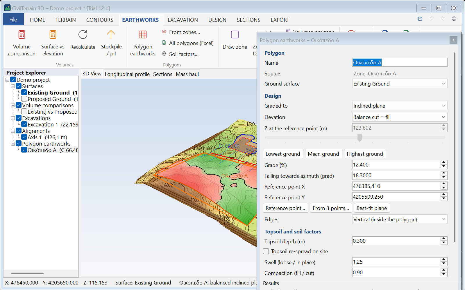
The plan shows the cut (red) / fill (green) map inside the polygon, the zero line and the daylight of the slopes. The item is saved in the project ("Polygon earthworks" node of the tree) and is recomputed automatically when the ground changes.
Buttons: Design surface (the plane as a surface for sections and comparisons; with slopes also the final ground), Surfaces inside the perimeter (below), As zone, PDF, Excel, DXF / DWG (outline with design elevations, zero line, daylight, texts) and Setting-out CSV (vertices and daylight with design Z, ground Z and ΔZ).
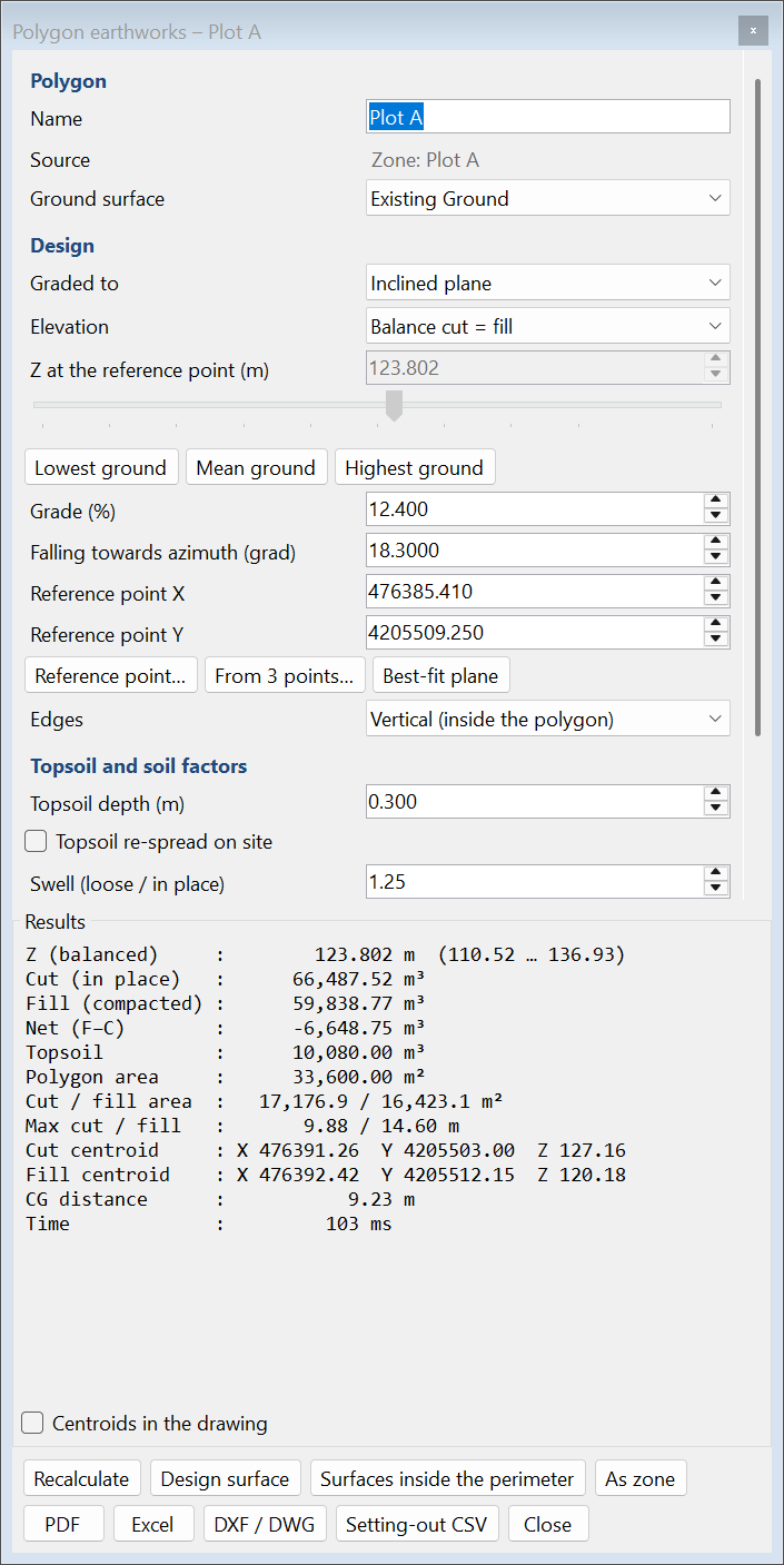
The window always opens inside the screen; on a small screen (e.g. 1366 × 768) it moves up or takes the whole height of the screen. The settings scroll, the results show whole lines and scroll when they do not fit, and the check box and the buttons are always in view.
Centroids of the volumes
The results also give the centroids (CG) of the cut volume and of the fill volume, e.g. for the haul distance of the excavated material:
- Cut centroid and Fill centroid: X, Y and Z. Z is the mean elevation of the volume, not a point of a surface: in an excavation of constant depth it lies at half the depth.
- CG distance: the horizontal distance between the two centroids, when both exist.
- They are the centroids of the volumes given as the result: after stripping the topsoil (the topsoil is a separate quantity and does not count in the cut centroid, while the fill also includes the stripped layer) and, with side slopes, including the slopes. The swell and compaction factors do not move them.
- Where there is no cut or no fill volume (up to 0.0005 m³), or where one is negligible next to the other (up to 0.01 % of it, e.g. 0.02 m³ of fill on the slopes of a 6,600 m³ excavation), its centroid and the distance read “—” (in Excel and in the item list the cell is left empty); its volume is still shown.
With the check box Centroids in the drawing under the results (or in the Properties), the centroids are drawn in plan and in the 3D view, at their position and elevation, over the surfaces: a red cross “CG cut”, a green cross “CG fill” and a thin line between them with the distance. The same crosses, line and distance also go on the plan of the PDF report. The box is not ticked by default and is saved with the item.
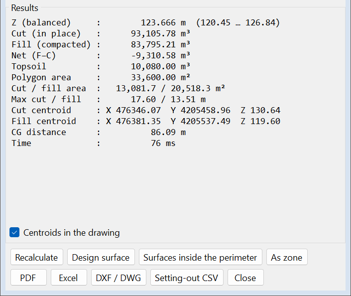
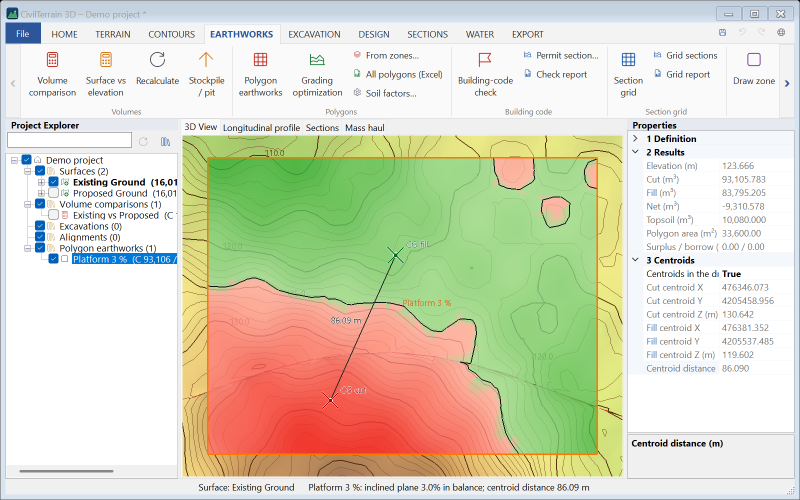
In the Properties of the item, the category 3 Centroids has the option “Centroids in the drawing” and the values Cut centroid X / Y / Z, Fill centroid X / Y / Z and Centroid distance. The PDF and Excel reports give them as “Cut centroid”, “Fill centroid” and “Distance between the centroids” (in Excel as numbers, X, Y and Z apart), with a paragraph on the method. The All polygons (Excel) table (section 12.9) and the item list (section 3.2) have them in columns.
Volume comparisons (section 12.2) give the same values, in the Properties, the item list and the PDF / Excel reports, with no drawing. With topsoil in the comparison, the Properties also give the centroids after stripping it, and the report, whose volumes are after the topsoil, gives those.
Surfaces inside the perimeter
The Surfaces inside the perimeter button (also in the right-click menu of the item in the tree) adds to the project two surfaces cut to the polygon: “… – ground inside the perimeter” and “… – design inside the perimeter”, with the name of the item in front. Depending on what the polygon is graded to, the design is the plane at the elevation of the result (e.g. after balancing), the piece of the other surface or the surface at the depth below the ground. A volume comparison of the two (section 12.1) gives the volumes and centroids of the item, and the surfaces serve for sections or exports of the polygon only.
- Both are added in one undo step.
- The copy of the ground is hidden, since it lies on the ground; so is the design when it is a piece of another surface. A plane or a depth shows in the colour of the “Design surface”.
- With side slopes the surfaces cover the polygon only: their comparison gives the part inside the polygon, without the slopes.
- With topsoil, the results of the item are after stripping the topsoil, while the comparison of the two surfaces gives them without stripping. The status bar says so.
12.7 Topsoil and soil factors
Topsoil: give a depth (e.g. 0.30 m). The topsoil is stripped over the whole works area before the earthworks, it is reported separately (a separate pay item that does not go into fills) and cut / fill are computed from the stripped ground. Topsoil can be set for polygon earthworks and for volume comparisons (Properties → "Topsoil depth"), so it also applies to the volumes per zone and the reports.
Soil factors (EARTHWORKS → Soil factors…):
| Factor | Meaning |
|---|---|
| Swell | Loose / in-place volume (e.g. 1.25): for haulage and truckloads. |
| Compaction | Compacted fill obtained from 1 m³ of cut (e.g. 0.90): for the balance. |
| Density | t per in-place m³ (e.g. 1.80): for the weight. |
| Truck | Capacity in loose m³ (e.g. 16): for the truckloads. |
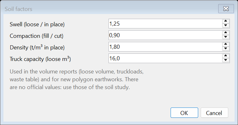
12.8 Balance, haulage and waste table
The reports of polygon earthworks and of volume comparisons contain a Balance and haulage table: loose volume and weight of the cut, material needed for the fill, cut reused on site, surplus to remove or borrow with loose volume and truckloads, and the topsoil.
A construction-waste (ΣΔΑ) table follows with category, EWC code (17 05 04 – soil and stones), in-place and loose volume, tonnes, reuse on site and removal — the data asked for in the waste management plan of a building permit. Check categories and quantities before submitting.
12.9 Several polygons at once
From zones… (or a DXF/DWG with several outlines): choose the polygons and a common design — level at the mean ground of each polygon, balance in each polygon or a common elevation — edges and topsoil. One item is created per polygon and at the end the All polygons (Excel) table is offered with volumes, topsoil, surplus / borrow, truckloads and totals. Overlapping polygons are warned about (the common area would count twice).
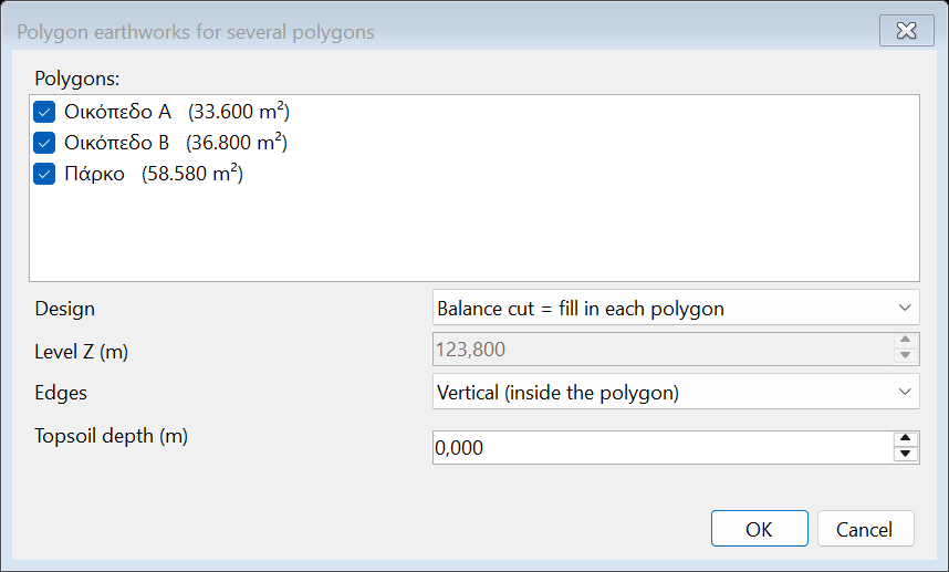
Sample: 10_zones_kyvismou.dxf (plots A, B and a park).
12.10 Final ground levels check (Greek building code, ΝΟΚ)
The Greek building code (ΝΟΚ, ν.4067/2012, now codified in ν.5306/2026) states that in the uncovered areas of a plot the final ground level at no point may be higher or lower than the natural ground by more than 1.50 m (art. 210 §4 and 212 §3a). On plots steeper than 20 % the ground may be lowered by up to 2.00 m and raised by up to 1.50 m. Works beyond these limits need an opinion of the Architecture Council. Excavations or fills of more than 0.80 m need a building permit (art. 315 §1c).
EARTHWORKS → Building-code check: choose the plot (zone, closed line, DXF/DWG, drawing or coordinates, as for polygon earthworks). In the window:
- Natural ground and final ground: surfaces of the project (e.g. the survey and the design / final construction surface). Where there is no final surface the ground is taken as unchanged (optional).
- Excluded areas: the building (the rule concerns the uncovered area) and everything that is not ground — ramps, stairs, cours anglaises, pools.
- Limits (editable): ±1.50 m, steep above 20 % with −2.00 / +1.50 m, permit threshold 0.80 m. Steep is decided from the plot slope or by the engineer.
- Plot slope: the law defines no method; the program gives the mean slope of the natural ground, the slope of its best-fit plane and the slope from its highest to its lowest point, and warns when they disagree about 20 %.
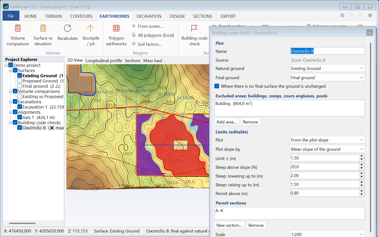
The result is exact at every point: both TINs are overlaid and every piece is split exactly at the limits. You get COMPLIES (green), LIMITS EXCEEDED (red) or NOT FULLY CHECKED (amber: part of the uncovered area has no natural or final ground — shown grey in the plan), whether a permit is needed, the largest lowering and raising with their coordinates, the areas per class, the volumes beyond the limits and the worst points (X, Y, natural Z, final Z, excess). Without a final ground surface (or if it is the natural ground itself) no verdict is given. A design exactly at a limit (e.g. exactly +1.50 m) counts as within it.
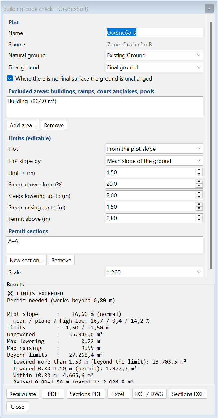
12.11 Permit sections
New section… (or Permit section…) draws the section line (two or more points; it may be bent). Sections PDF gives each section on its own page at 1:100, 1:200 or 1:500 (same horizontally and vertically, as the coverage diagram requires — art. 325 §3ε), with the natural ground (dashed), the final ground, the allowed range, the parts beyond the limits in red (only inside the plot and outside the buildings), the building and the plot boundary. The scale is saved with the check and is also used for the sections in the PDF report. If a section does not fit at the chosen scale, the next one is used (paper up to A2). Sections DXF gives each section as a CAD drawing in real metres (X = station, Y = elevation) for the coverage diagram; with several sections one file per section is written (“<name> A.dxf”, “<name> B.dxf” …).
The PDF report has the check data, the plan of the classes with the points and section lines, the text of the provision and all sections. Excel and DXF / DWG (plot, excluded areas, limit lines, points, sections) are also available.
12.12 Section grid and volumes
The section grid gives the classic volume computation with parallel cross sections (e.g. for dredging to a design level, the excavation of a yard or a regrading): sections every d m inside a boundary, perpendicular to a baseline, grid nodes with the ground elevation and Δh, cut / fill areas per section and volumes by the average end area method.
- EARTHWORKS → Section grid (or SECTIONS → Section grid). A selected zone or closed line becomes the boundary; otherwise choose the outline of the surface, click an outline, draw it, or take it from DXF/DWG or coordinates.
- In the grid window set the ground surface, the design level (e.g. −5.00 m) or a design surface, the distance between sections and the distance between nodes. The baseline follows the long side of the boundary (smallest enclosing rectangle) or an azimuth in grads.
- The grid is drawn on the plan: boundary, sections S1, S2 … with their names, node lines, nodes with Δh (+ = cut) and the cut / fill map. Every change is recomputed at once.
- Sections: the sections appear in the Sections tab with their names; the current one is highlighted on the plan.
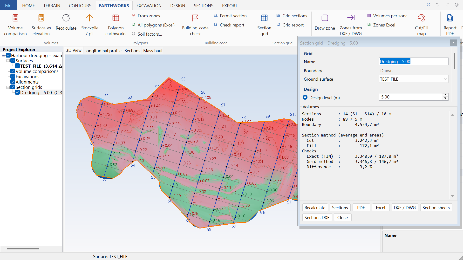
The results are given in three ways, as checks:
| Method | Description |
|---|---|
| Sections (average end areas) | The areas of every section are exact between the ground and the design line; the volume between two consecutive sections is half the sum of their areas times their distance. The first and the last section lie at the ends of the boundary. |
| Exact TIN volume | The volume of the TIN prisms inside the boundary (no approximation). |
| Grid method | The mean Δh of the four corners of each cell times its area; Δh at the centroid for the cells on the boundary. |
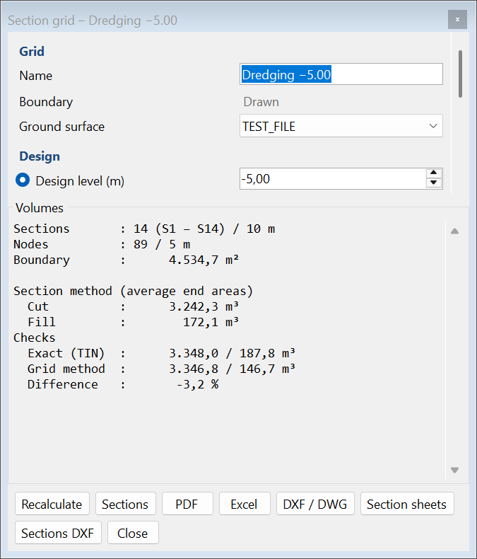
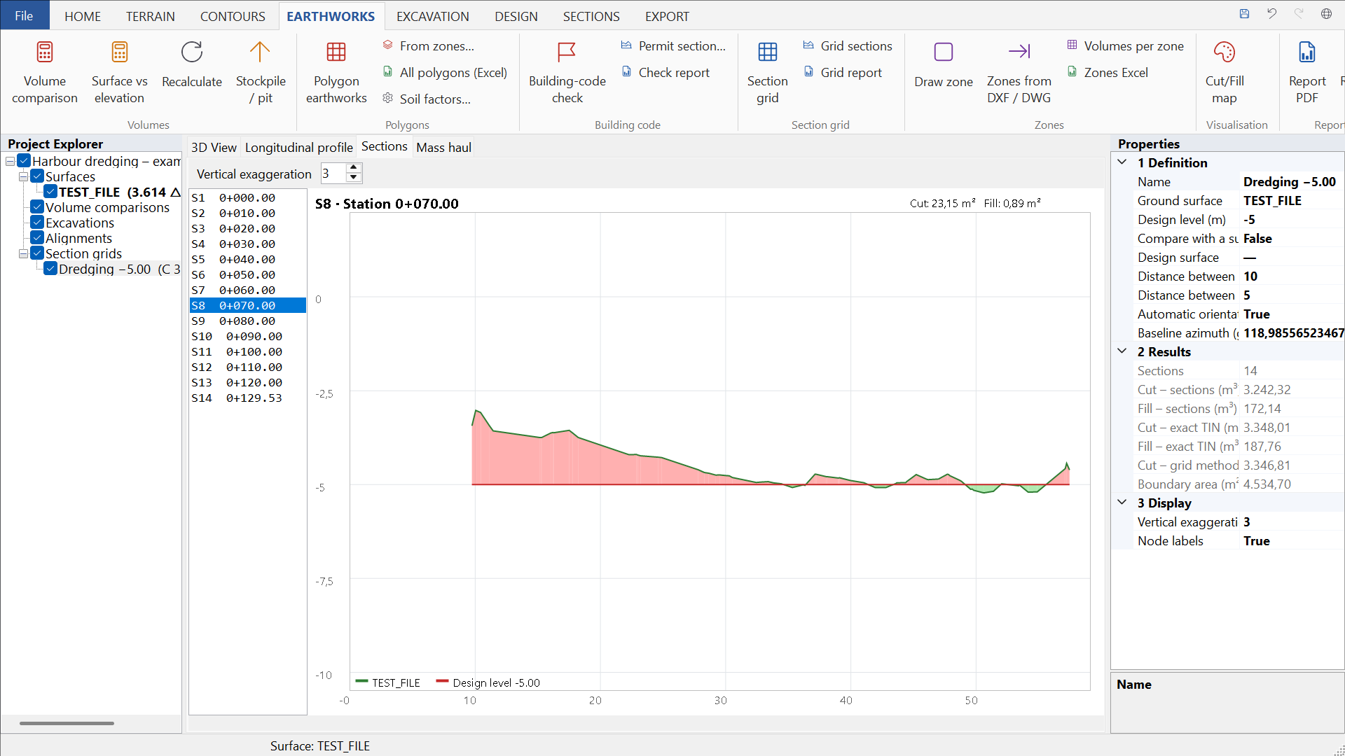
Exports: PDF (summary, volume table, A3 plan with contours, all sections at a common scale and the node table), Excel (volumes, nodes, cells, section points), DXF / DWG (boundary, named sections, node lines, nodes with Z and Δh), Section sheets at scale and Sections DXF.
12.13 Δz labels on a grid (cut / fill map with height differences)
The height differences Δz are written over the cut / fill map of a comparison at the nodes of a regular grid, at the spacing you give (e.g. every 10 m) — like the maps of height differences delivered in AutoCAD.
- Select the comparison in the tree (otherwise the last one is used).
- EARTHWORKS → Visualisation → Δz labels on a grid… and type the node spacing (m). 0 removes the labels.
- The spacing can also be changed in the comparison Properties: Δz labels every (m, 0 = none).
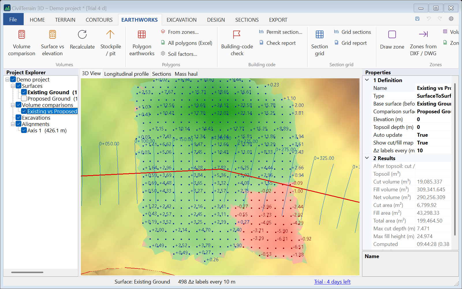
- Δz = after − before (comparison − base surface, or elevation − surface): + fill (blue), − cut (red), with two decimals.
- The nodes lie on round coordinates (multiples of the spacing), only where both surfaces exist. Where the surfaces coincide (Δz = 0.00) no label is written.
- On screen, labels that would overlap are left out and appear as you zoom in.
- The Volume report PDF writes the differences on the cut / fill plan, and the Excel file adds a Δz grid sheet with X, Y, base Z, comparison Z and Δz of every node.
- EARTHWORKS → Δz map DXF / DWG: cut / fill faces (layers CF_CUT, CF_FILL), nodes (CF_NODES) and Δz texts (CF_DZ_CUT, CF_DZ_FILL) with a text height in proportion to the spacing.
13. Dynamic excavation design
Draw the outline of an excavation (or pad) and the program creates the 3D surface with slopes that intersect the real ground geometrically. The final top outline (daylight line) results from this intersection, not from a constant horizontal offset.
- Make the ground surface active.
- EXCAVATION → New excavation and draw a closed outline.
- The Excavation designer opens.
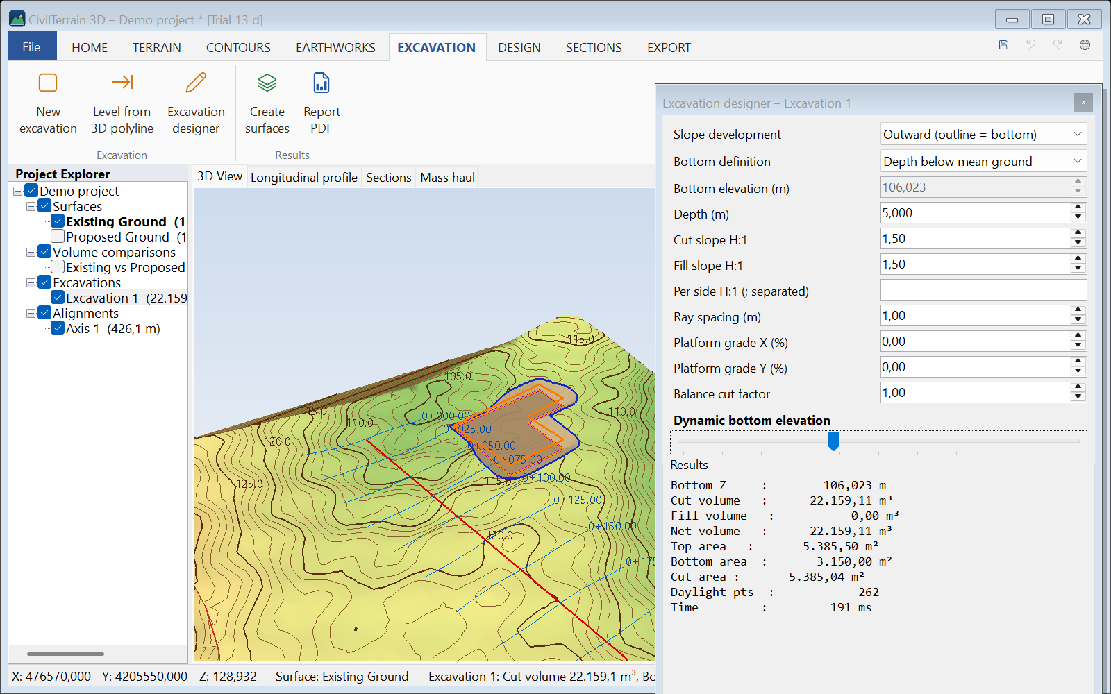
| Field | Description |
|---|---|
| Slope development | Outward: the outline is the bottom and the slopes rise outwards to the ground. Inward: the outline is the top edge on the ground and the slopes go down inwards. |
| Bottom definition | Absolute bottom elevation or depth below the minimum / mean / maximum ground elevation along the outline. |
| Cut / fill slope H:1 | Horizontal to vertical (e.g. 1.5 = 1.5 horizontal to 1 vertical). Where the bottom is above the ground, an embankment with the fill slope is created. |
| Per side H:1 | Different slope per side, separated by ; (1st value for the side from vertex 1 to 2, etc.). Empty = same for all. |
| Ray spacing | Spacing of the computation points along the outline (smaller = more accurate). |
| Dynamic bottom elevation | Slider: while dragging you see a fast preview; when released the exact calculation is done. |
Results (bottom elevation, cut/fill volumes, top/bottom areas, time) update immediately. Create surfaces adds the Excavation Surface and the Final Construction Surface (ground + excavation) to the project, plus a volume comparison. Redraw outline lets you draw a new outline.
14. Feature lines, platforms and grading optimization
The DESIGN tab contains grading tools in a simple form.
14.1 Feature lines
3D lines with editable elevations: curbs, ditches, platform edges, walls. Create them with Feature line / Closed line (elevations from the active surface), From breakline or automatically from point codes. 3D lines also come from the 3D polylines of a DXF / DWG, without a surface (section 15.7). Click a line and its Properties show its weighted slope, name, colour and visibility (the last three can be changed there).
In Edit elevations:
- vertex table with distance, X, Y, Z and grade to next — edit Z or grade directly;
- Elevations from surface, Interpolate between selected, Constant grade…, Raise / lower…;
- a small profile of the line (orange) with the ground (green dashed);
- Breakline of a surface: the line enters the TIN and every elevation change updates the terrain automatically.
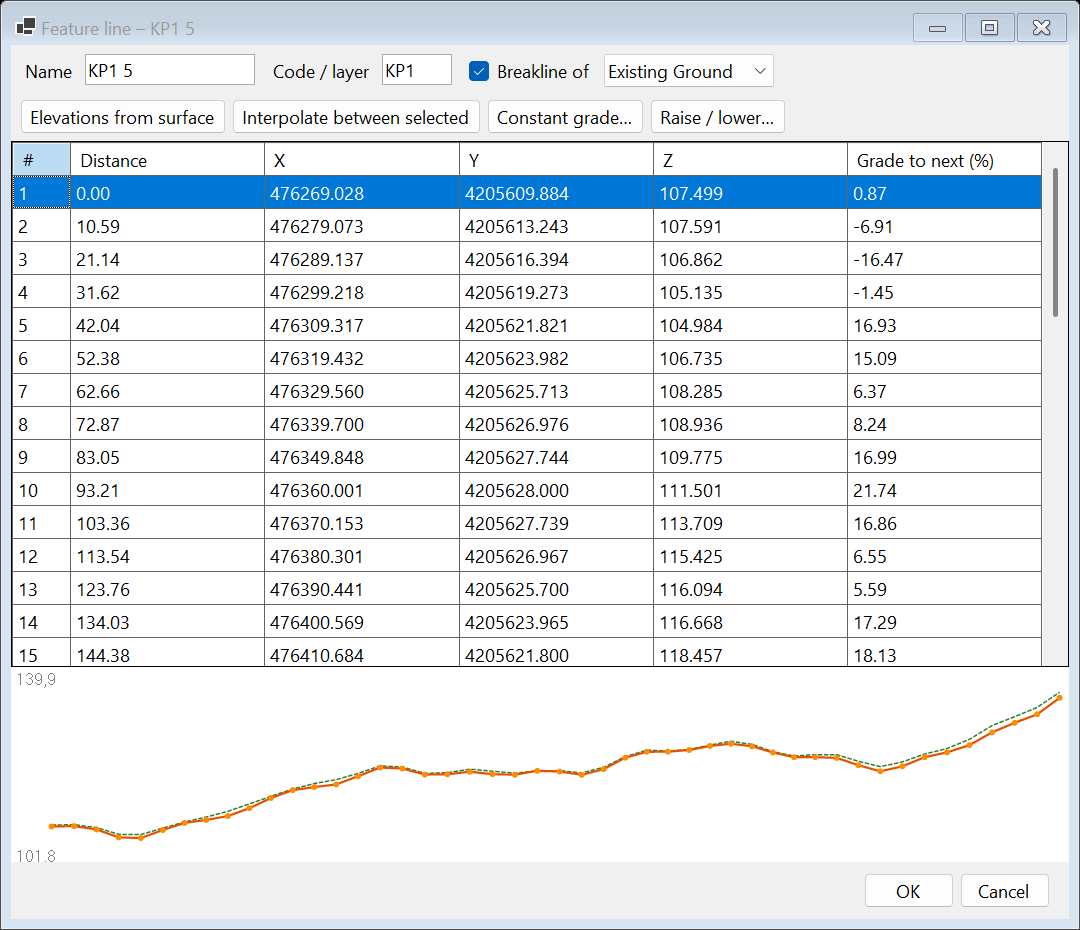
14.2 Platforms with earthwork balance
Platform: draw the outline; the designer opens with extra platform grades X / Y (%). Cut/fill slopes develop outwards to the ground. Platform from line: the platform edge follows the elevations of a closed feature line (e.g. with drainage grades).
Balance cut = fill finds the elevation for which cut × factor = fill (zero balance, no import/export of soil). The factor expresses swell/shrinkage (e.g. 0.9) and is saved with the platform. Ideal for plots, solar parks, sports grounds and warehouses. For topsoil, an inclined plane by azimuth or a required surplus use polygon earthworks (with "side slopes to the ground").
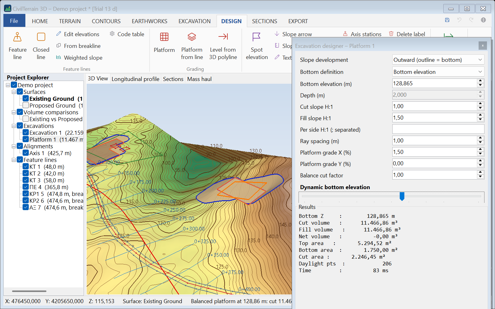
14.3 Cut-and-fill level from a 3D polyline
When the level is already drawn in CAD, import it directly: DESIGN → Level from 3D polyline (or EXCAVATION) and choose a DXF or DWG file and layer.
- The largest closed 3D polyline (3DPOLY) becomes the outline with the elevation of each vertex (grades, different levels).
- Polylines inside the outline become grade breaks of the level (ridges, valleys, grade changes).
- The level can be above and below the ground at the same time: where the ground is higher a cut slope is created, where it is lower a fill slope.
- In the designer the slider and Balance cut = fill move the whole level (outline and interior lines) keeping its grades.
Sample: 09_epipedo_3dpoly.dxf (60×40 m platform with 2% grade and a ridge).
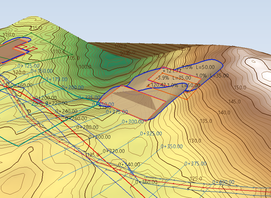
Level accuracy: outline vertices on a straight edge keep their elevation (e.g. a gable), interior lines are clipped exactly at the outline, and where a grade break touches the outline (or stops up to 5 cm short of it) it becomes an outline vertex, so the surface and the slopes have one elevation at every point. "Redraw outline" replaces the 3D level by a horizontal bottom at its mean elevation.
14.4 Grading optimization inside an outline
EARTHWORKS → Grading optimization: inside an outline the program finds the surface with the least earthworks that keeps your criteria. It needs only the largest grade (e.g. not above 5%) and, if you wish, where the water should go.
- Outline: click a zone, a closed line or an outline, draw it, take it from a DXF / DWG or type coordinates, as for polygon earthworks. A zone or closed line selected in the tree is used directly.
- Criteria: the criteria dialog opens at once (below).
- Compute: in a few seconds you get the design surface and its comparison with the ground, with a summary of the results.
| Criterion | Description |
|---|---|
| Largest grade (%) | The grade of every triangle, in any direction, stays within this value. |
| Water path | Draw a water path…: the dialog hides and you draw a line from high to low (Enter to finish). Around each of its segments the ground falls in its direction at least at the smallest fall (e.g. 1%). Draw as many paths as you need. |
| Outlet (manhole) | Click where the water is collected. All around it the ground falls towards it. |
| Points of given elevation | Click in the drawing and type the elevation, e.g. an entrance, a building threshold, a manhole. |
| Lowest / highest elevation | Optional limits for the whole surface, e.g. above a flood level. |
| Deepest cut / highest fill | How deep it may dig or how high it may fill (0 = no limit). |
| Balance | Fill = factor × cut, side slopes included. |
| Cut / fill side slopes | The slope (H:1) that ties the surface to the ground outside the outline. |
| Grid spacing | 0 = automatic (about 20,000 nodes). A denser grid gives more detail and takes longer. |
| Accuracy | Fast (recommended, up to ~20 s), Normal (within 2% of the least earthworks, up to ~1 minute) or High (within 0.5%, up to ~3 minutes). In practice "Fast" gives volumes just above the least. Esc cancels the computation. |
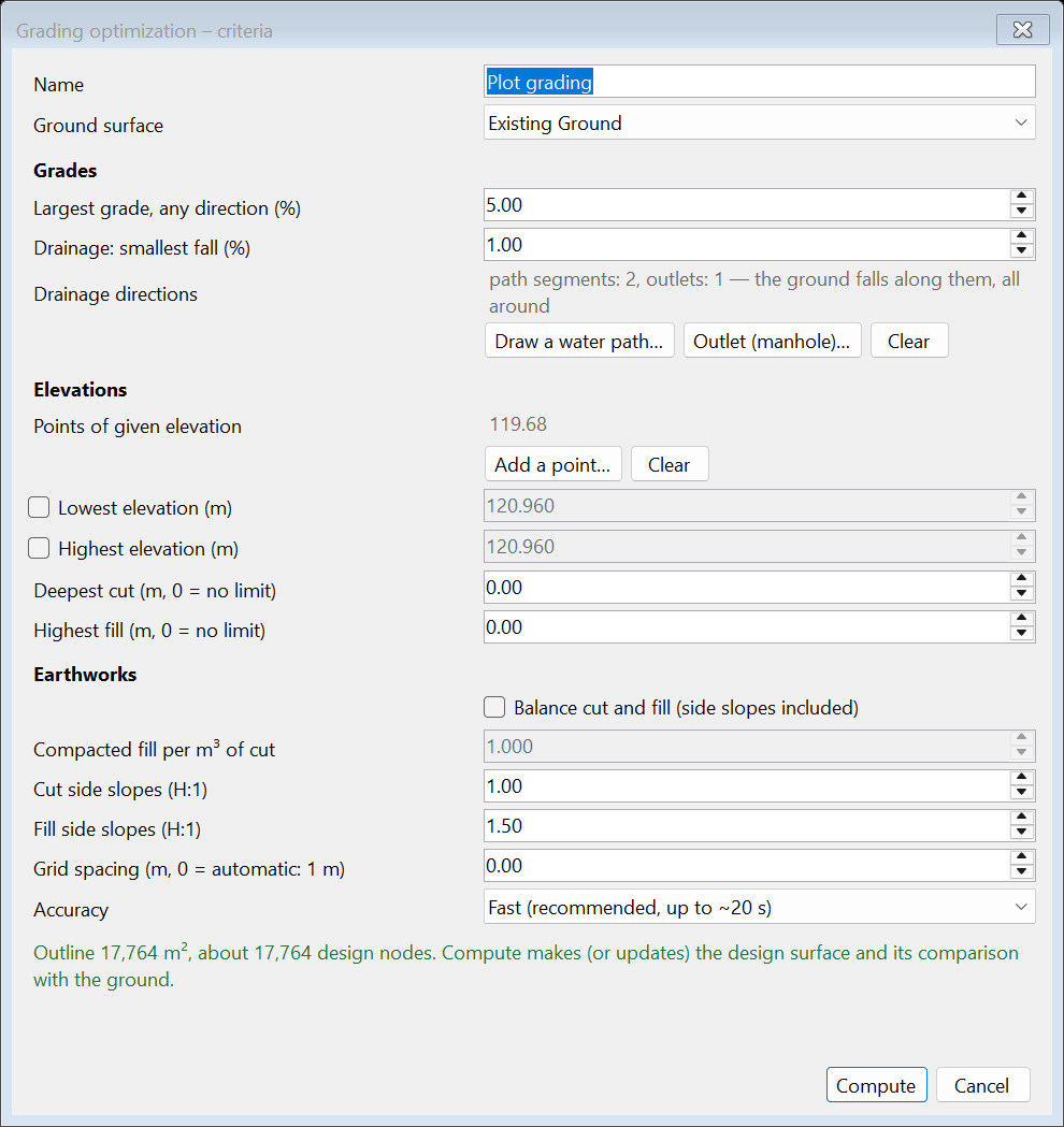
Result. The design surface is coloured in grade classes that end at the largest grade and has contours every 0.25 m. The blue arrows show where the water runs. The comparison "ground → design" gives the cut / fill map, the reports and the Δz labels. The summary shows:
- cut, fill and net, exact between the two TINs;
- how they split between the inside of the outline and the side slopes;
- the largest grade reached, the share of the area that drains correctly, and the balance;
- how close the solution is to the least possible earthworks, with a bound certified by mathematical duality.
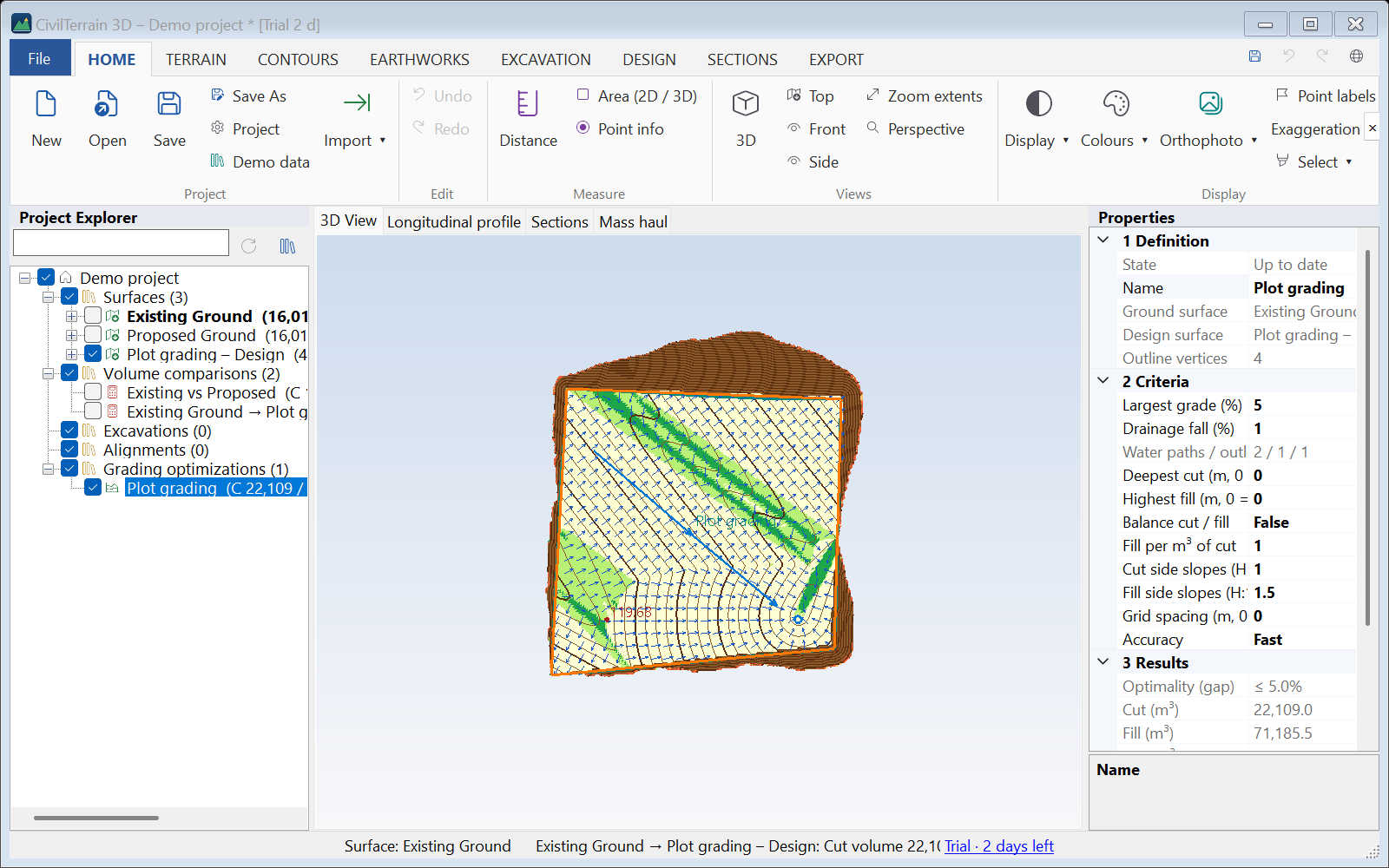
Changes. Change the criteria from the tree (Criteria…) or in Properties. After a change the optimization shows as out of date (⚠), as it also does when the ground changes. Recalculate updates the same design surface (with undo) and the same comparison.
14.5 Sloped design (sub-areas)
DESIGN → Sloped design: inside the perimeter of a site you draw sub-areas of any shape and give each side a grade % as you draw. They make a new design surface, with side slopes to the ground, and its comparison with the ground: volumes and cut / fill colours. Both update as soon as anything changes, so you see at once whether a layout pays off.
- Perimeter: select a zone, a closed line or an outline in the tree before the command. It is shown dashed and vertices snap onto it. With nothing selected, the design starts without a perimeter.
- Drawing an area: click its vertices.
- In the small window you give the grade of the next side (+ uphill, − downhill, in the direction you draw) and you can change it before every click.
- The 1st vertex takes the elevation of the ground, or one you type.
- For the point under the cursor, the window shows the length, grade and elevation of the side, and the closing side.
- Enter or a double click: the area is done; Backspace: back one vertex. A click on the first vertex again snaps onto it.
- In the grade box both a point and a comma are a decimal point; Enter there keeps the value and goes back to the drawing.
- Neighbouring areas: a click on a vertex or side of another area makes a shared point at its elevation, so the areas join without steps. After each area the drawing goes on with the next one; Esc ends it.
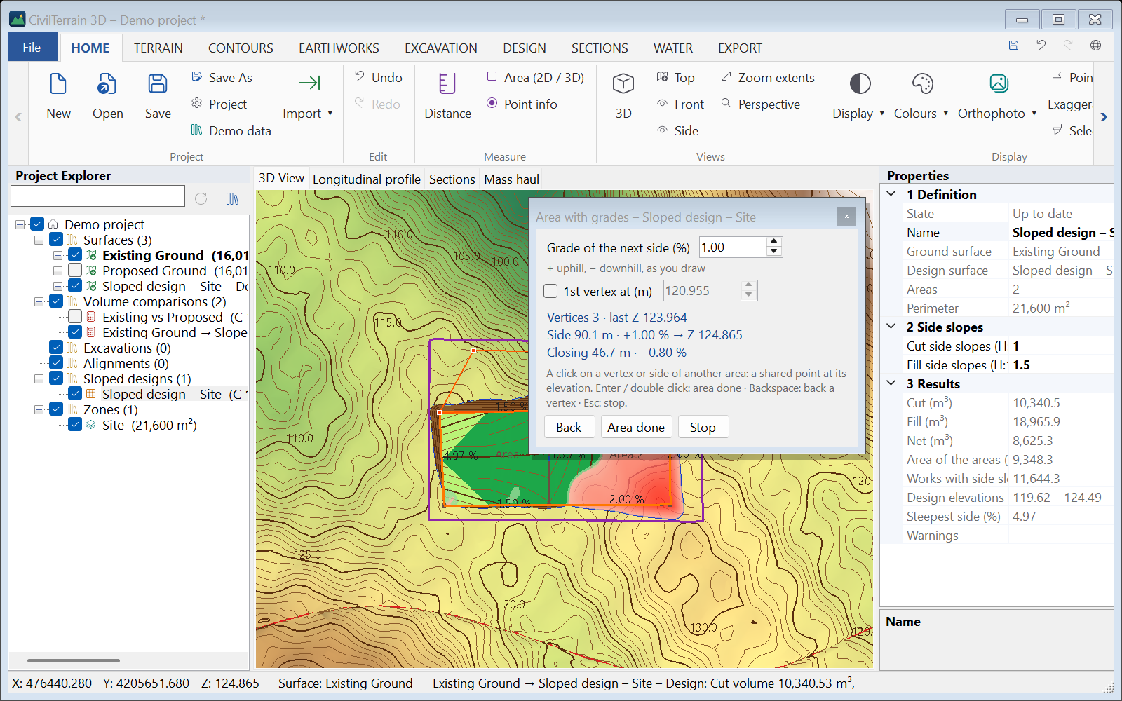
Result. The areas join into one design surface. Its outer edge meets the ground with the cut and fill side slopes of the Properties (e.g. 1:1 and 1.5:1). The drawing shows:
- the grade of each side, with an arrow pointing downhill;
- the cut (red) and fill (green) colours.
The Properties and Results… give:
- cut, fill and net;
- the area, and the works area including the side slopes;
- the range of elevations and the steepest side;
- the volumes per area, and of the side slopes on their own.
A gap enclosed by areas (a courtyard, say) is designed from the areas around it; a warning tells so and its volumes are in the row «Gaps between areas». Areas that overlap or cross themselves (vertices out of order) are pointed out.
The Excel export contains the volumes and the vertices.
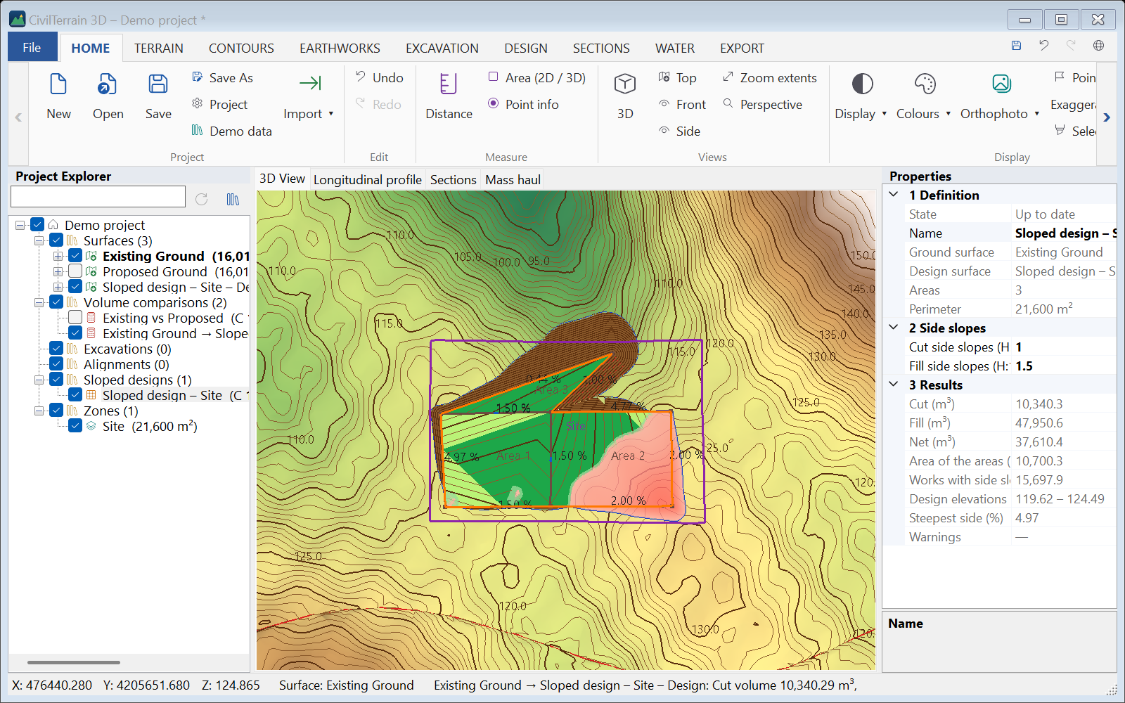
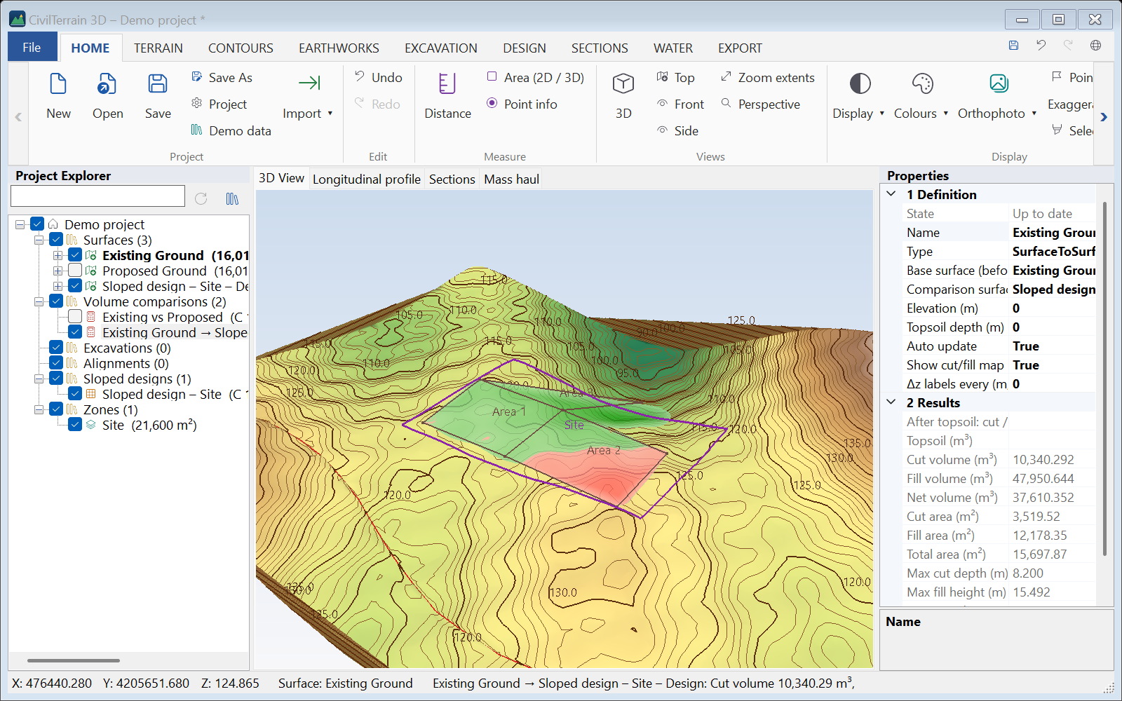
Changes. Right-click the design → Areas (elevations, grades)…: a table with the elevation of every vertex and the grade of every side, the closing side included.
- A changed grade moves the next vertex. With the box ticked, the vertices after it move too, so their own sides keep their grades.
- Points shared with other areas follow. A point lying on a side of another area (not on one of its vertices) does not follow; if it ends up at another elevation than that side, a warning says so and the side bends there.
- In the same table you rename or delete areas.
New areas are drawn with right-click → Draw an area…. Every change is undone with Ctrl+Z, and the design surface updates by itself.
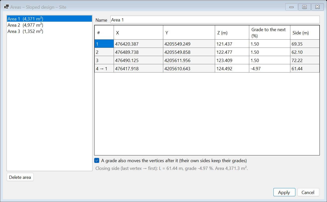
- The design surface belongs to the design: every change of the areas makes it anew, so manual edits on it are lost. Until then the design shows as out of date (⚠), since its figures no longer describe the surface.
- When the ground changes, the design shows as out of date (⚠) until you Recalculate it.
- If the vertices of an area do not lie in one plane, its surface folds along a diagonal.
- Areas reaching the edge of the survey keep their elevations up to it; side slopes and volumes are computed only where there is ground (a warning says so).
15. Axes, profiles and cross sections
15.1 Drawing an axis
SECTIONS → Draw axis: draw the axis polyline. The sections dialog opens immediately.
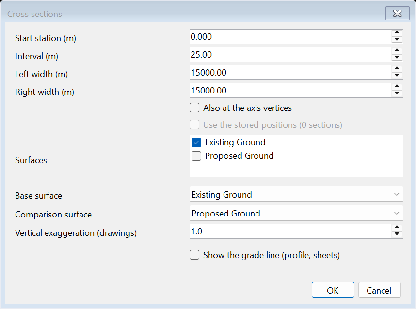
| Setting | Description |
|---|---|
| Start station | Chainage of the start of the axis. |
| Interval | Section spacing (e.g. 20 m, up to 15 000 m). Start and end are always included. |
| Left / right width | Length of the section on each side of the axis (up to 15 000 m). |
| Also at the axis vertices | Adds sections where the axis changes direction. |
| Use the stored positions | For axes imported from a positions file (chapter 16). |
| Surfaces / base / comparison | Which surfaces are drawn and between which the cut/fill areas are computed. |
| Show the grade line | Whether the grade line (design profile) is drawn on the profile and the sheets. Without it only the ground data remain; its VIPs are kept. |
The sections are also shown on the plan: blue lines labelled with their chainage. The section selected in the list is highlighted in orange.
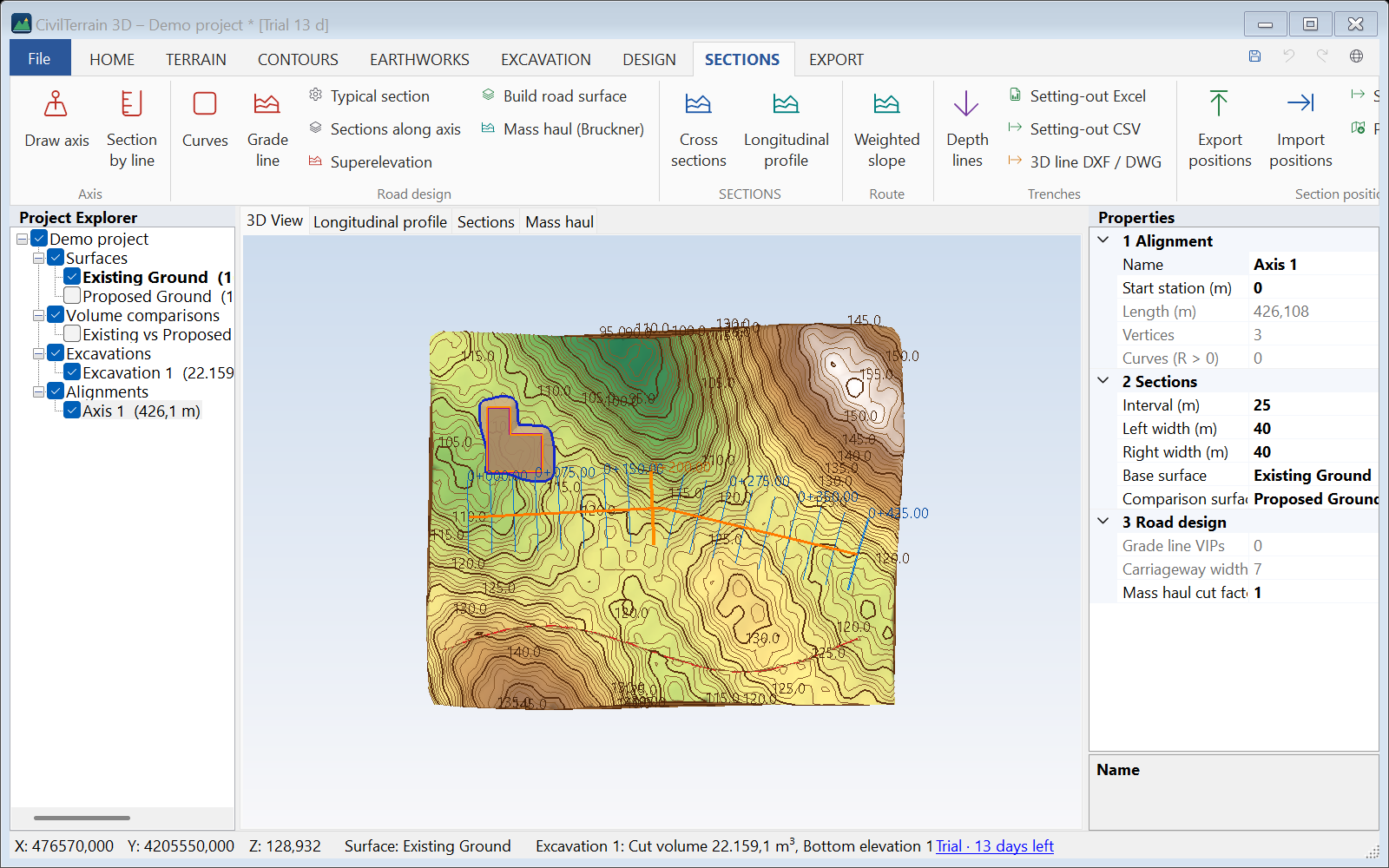
15.2 Longitudinal profile
The longitudinal profile has its own tab (SECTIONS → Longitudinal profile). It shows the surfaces along the axis, cut/fill shading, the axis vertices (V) and a band table with chainages, ground and design elevations and their difference. The band is written at the section stations or at a fixed spacing (Band every). Vertical exaggeration is set at the top left.
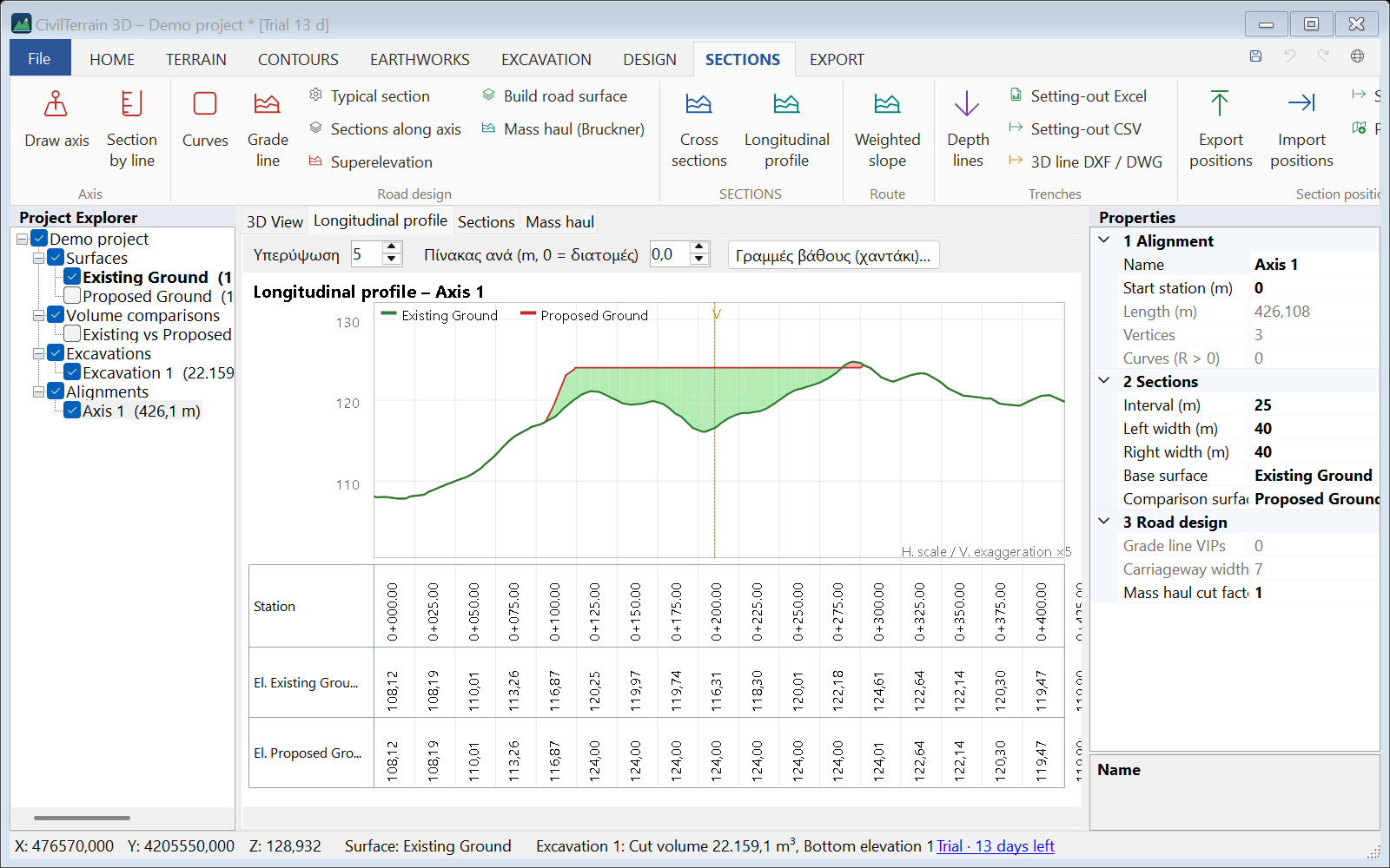
When the axis has a grade line, the Grade line box above the profile shows or hides it. Hidden, it is not drawn on the plan-profile sheets either and its VIPs cannot be dragged; the band shows only the ground. The same option is in the sections dialog and in the axis Properties.
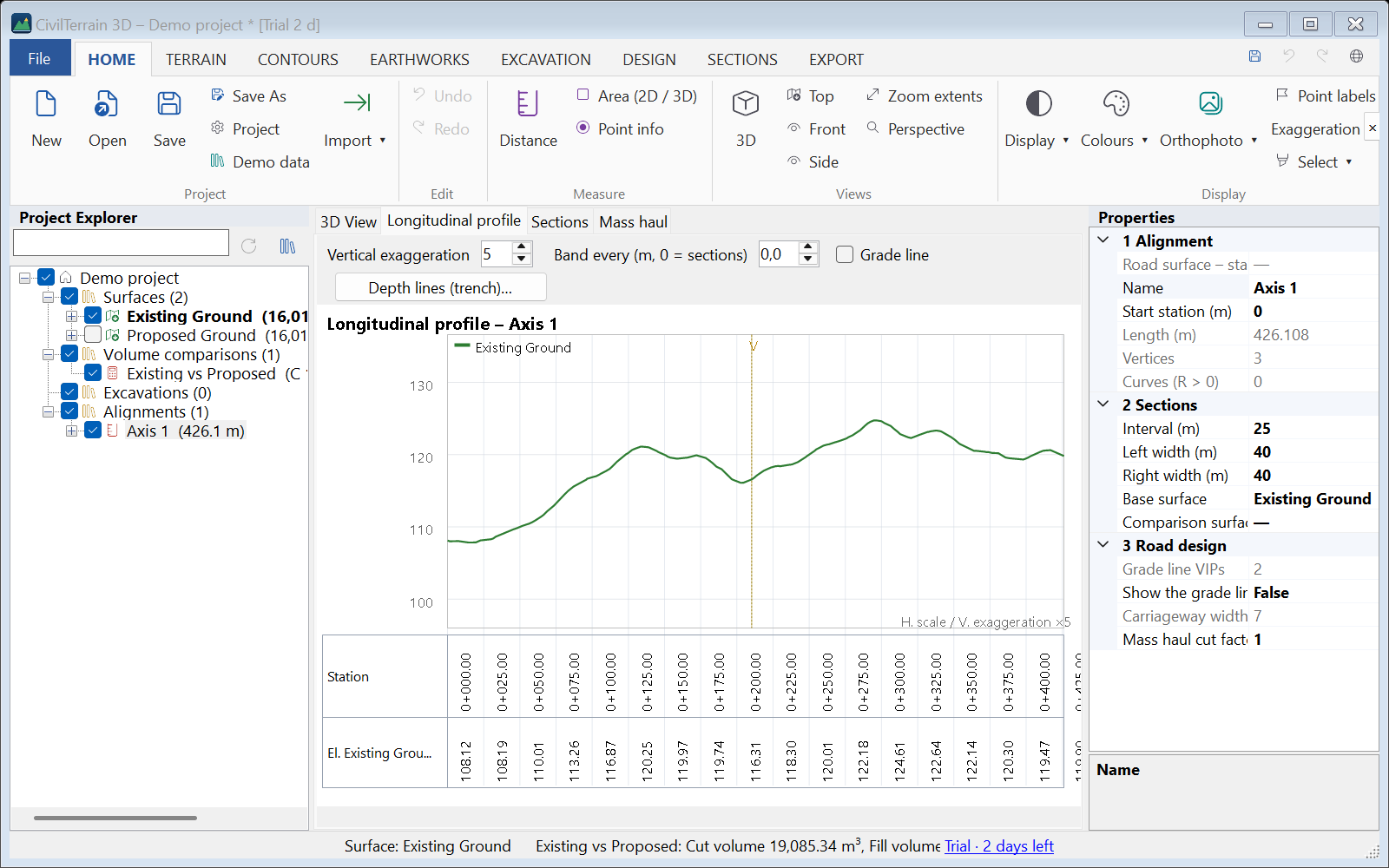
15.3 Cross sections
On the Sections tab pick a chainage from the list. Each section shows the surface profiles, the axis (red dashed), cut/fill shading and areas. Move the cursor to read offset and elevations.
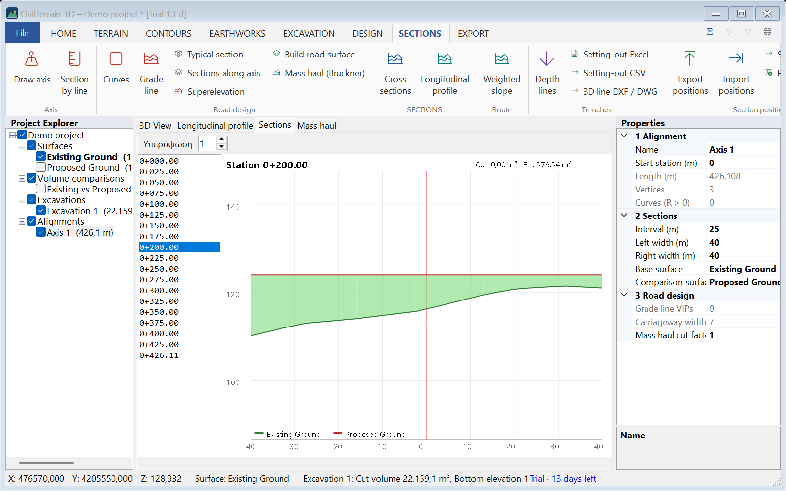
Volumes between sections use the average end area method and appear in the reports. For the exact volume also use the surface comparison (chapter 12).
15.4 Section by line
SECTIONS → Section by line: two clicks show the profile of all visible surfaces along that line.
15.5 Depth lines (cable and pipe trenches)
For cables, pipes and networks: SECTIONS → Depth lines (or the Depth lines (trench)… button above the profile). Each line has:
| Item | Meaning |
|---|---|
| Depth | E.g. 1.20 m for the cable and 1.30 m for the trench bottom — as many lines as you need. |
| Below | ground (follows the terrain) or grade line (follows the design; the actual depth below ground is shown separately). |
| From / To station | Part of the axis (empty = all). For different depths in different parts define more lines. |
| Width, wall slope | Trench section (rectangular or trapezoidal) for the excavation volume, shown per line and in total. |
| Indications every (m) | How often a depth indication is shown (e.g. 10, 20, 25 m); always at the start/end of the line too. |
In the profile the lines are dashed, with a vertical mark from the ground down to the line and the depth written next to it. The band under the profile gets the elevation and the depth of each line at the indication stations. The same appears in Profile PDF and Plan-profile sheets.
Exports: Setting-out Excel (length/volume summary and a setting-out table per line), Setting-out CSV (with X, Y of every indication for GPS) and 3D line DXF / DWG (the trench bottom as a 3D polyline on the axis, with labels).
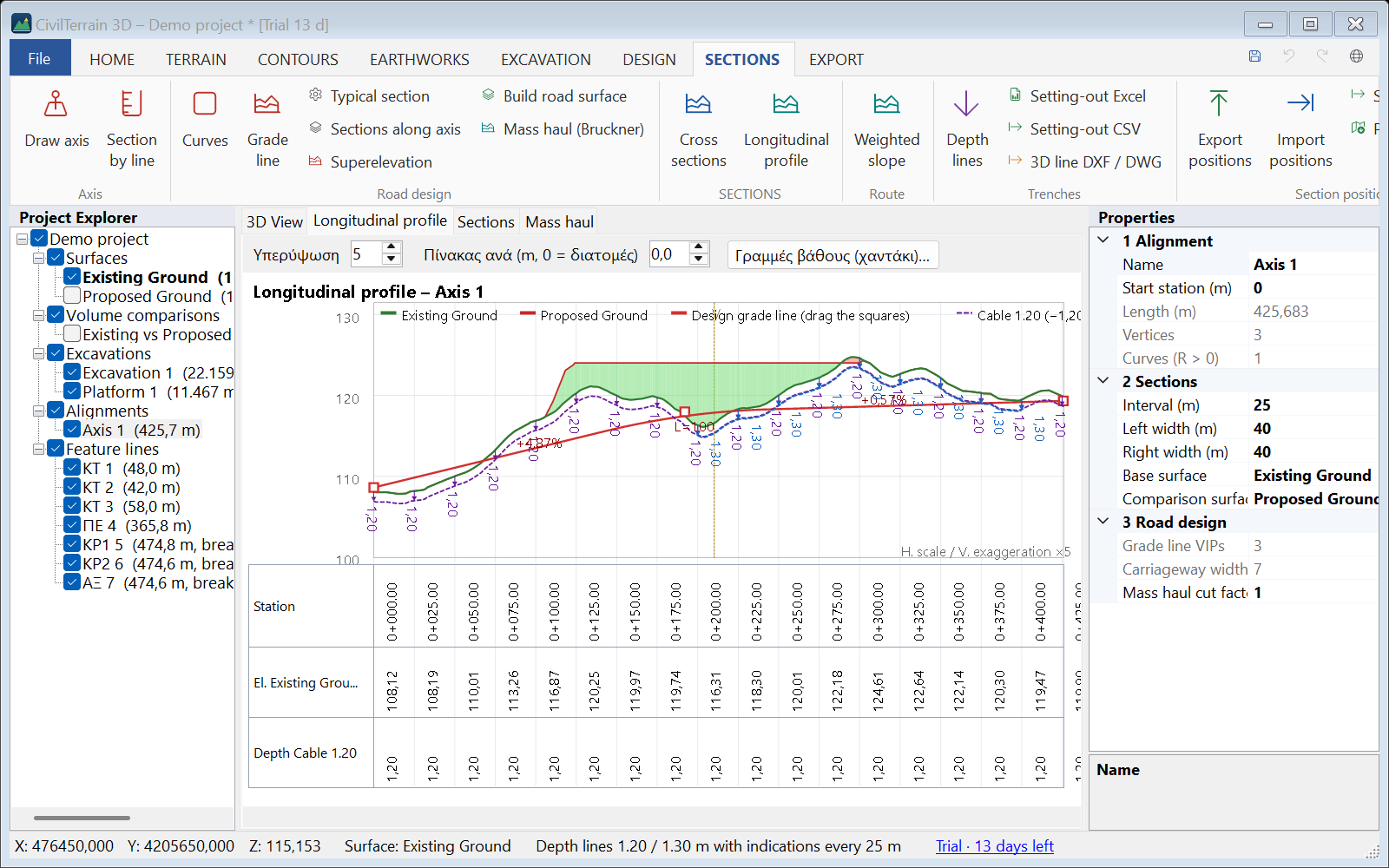
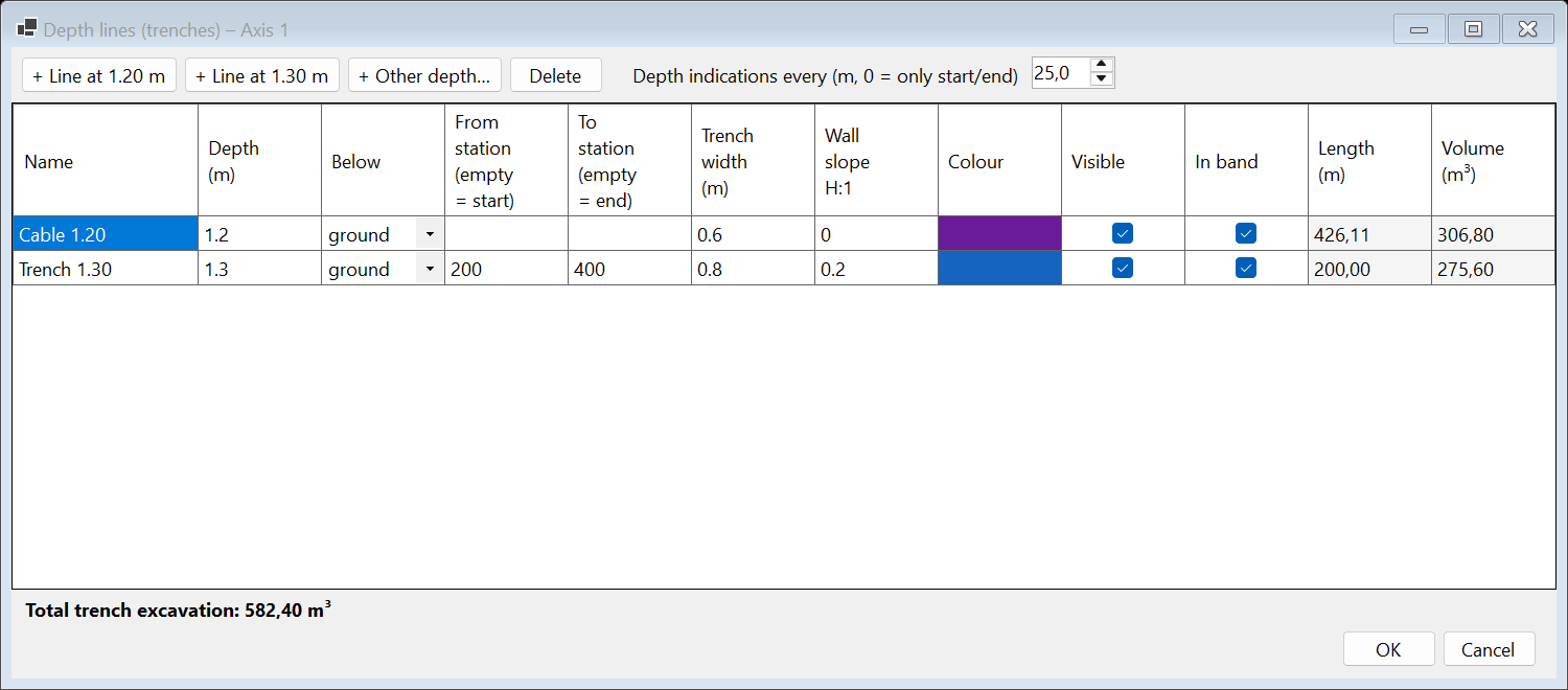
15.6 Weighted slope of a route
SECTIONS → Weighted slope (also in DESIGN or the axis right-click menu). It computes the weighted slope of a route (road, network, cable) as in the classic spreadsheet:
Weighted slope = Σ ΔHv / total horizontal length
(ΔHv = uphill height differences only)
Source of the points:
- Axis on the ground every N m (e.g. 20 m); with 0 every slope change of the terrain is used (exact value).
- Feature line: its vertices in order.
- Points file CSV/TXT in route order (No., X, Y, Z).
- Line of the drawing (click): click a 3D polyline you imported (from DXF / DWG, as a breakline of a visible surface) or a feature line, and the X, Y, Z of its vertices are taken directly — no ASCII file needed.
To pick by clicking: SECTIONS → Of a line (click), or Pick in the drawing… in the weighted slope window. Click near the line; the window opens with its name, the line is highlighted in the drawing and the result is computed at once. Closed lines are computed back to their first point.
The line is found where it is drawn on the screen, so Of a line (click) also works without a surface, e.g. on routes imported as 3D lines only (section 15.7). Quicker still: right-click a feature line, in the tree or in the 3D view, → Weighted slope…, and the window opens for that line. The window starts with the first source available, in this order: the line you clicked, else the selected line, else the axis, else the first line of the project, else a points file.
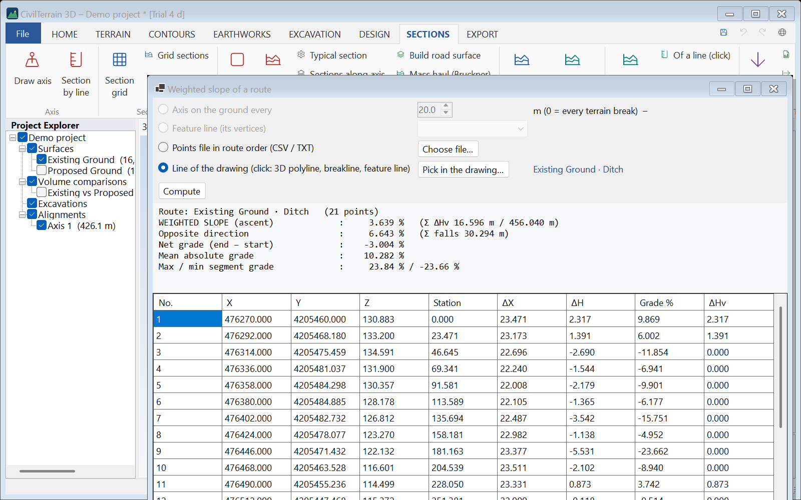
Shown: weighted ascent, the value in the opposite direction (Σ falls / length), net grade (end − start), mean absolute grade and max/min segment grade, with the table No., X, Y, Z, Station, ΔX, ΔH, Grade %, ΔHv. Export to Excel (same layout as the classic sheet) or CSV. Sample: 11_diadromi.csv.
In the window, next to Compute, two buttons lead to the routes without a surface (section 15.7): Import routes (DXF / DWG)… and Weighted slope of all lines….
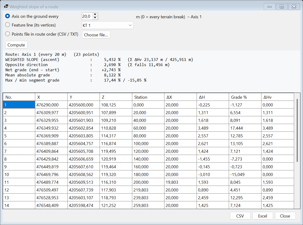
15.7 Routes without a surface – weighted slope with one click
Many routes (roads, networks, cables, several km long) that you have as 3D polylines in a DXF / DWG need neither a surface nor a points file each. Every polyline is imported as a 3D line of the project with its own vertices, and one click on it shows its weighted slope (Σ ΔHv / horizontal length, section 15.6) in the Properties. All of them together give one table with totals and export to Excel / CSV.
Import
- SECTIONS → Route → Import routes… and choose the DXF or DWG. The same command is the Import routes (DXF / DWG)… button of the weighted slope window and is also in the right-click menu of Feature lines in the tree. With the normal import (HOME → Import ▾ → DXF…) tick 3D polylines as 3D lines only (no surface) to do the same (section 7.2).
- In the Import routes (DXF / DWG) window choose the Layers. The surface options are not shown here. Layers without any polyline with elevations (e.g. a frame or a title block of 2D lines, like FRAME of the sample
13_diadromes.dxfin Figure 15.9) start unticked when another layer has routes; tick them if you want them. - In Source CRS set the system of the file if it is not the project's (default “Same as project (no transformation)”). In an empty project, a projected system (e.g. GGRS87, UTM) becomes the project's system. Files in geographic coordinates (longitude / latitude) or Web Mercator are always transformed into the project's system, because the lengths of the slope are measured in metres, in the plane.
- Click OK. After “Import routes” the Weighted slope of all lines table opens at once as well (below).
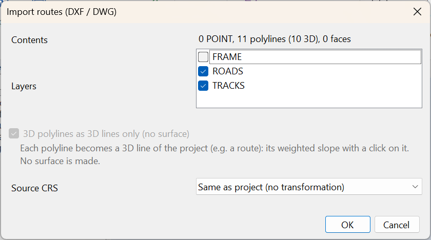
No surface is made. Every polyline becomes a 3D line named after its layer with a running number, in the order of the file: for the layer ROADS, “ROADS 1”, “ROADS 2” … (just “ROADS” when the layer has one line; for layer 0, the file name). A name already in the project gets “(2)”. The code of the line is its layer, each layer has its own colour, and closed polylines stay closed. The view goes to the new lines, and the whole import is undone with one Undo.
The status bar says how many lines came in. Lines without elevations (every vertex at one Z, e.g. 2D polylines) have a weighted slope of 0 %: the program warns about them once, with their names. Polylines of a single point are left out. Vertices with invalid coordinates are skipped, and the message says how many. 3D polylines with a spline fit are read by the points of their fitted curve (the control points of the frame are ignored). If the project is in degrees (longitude / latitude), the message asks you to set a projected system (e.g. GGRS87) for lengths in metres. If the coordinates of the file look like degrees while Source CRS is “Same as project”, a warning appears: undo (Ctrl+Z), choose WGS 84 (lon/lat) in Source CRS and import again.
One click: the weighted slope in the Properties
Click a route in the 3D view or in the tree. The line is selected and the Properties show the result in the 1 Weighted slope group, from its vertices in order, with no surface:
| Field | Meaning |
|---|---|
| Uphill (%) | The weighted slope in the direction of the line: Σ rises / horizontal length. |
| Opposite (%) | The weighted slope in the opposite direction: Σ falls / horizontal length. |
| Length (m) | The horizontal length of the line. |
| Σ rises (m) | Σ ΔHv: the sum of the rises along the line. |
| Σ falls (m) | The sum of the falls along the line. |
| Net grade (%) | (Z end − Z start) / horizontal length. |
| Mean |grade| (%) | Mean absolute grade: (Σ rises + Σ falls) / horizontal length. |
| Max / min (%) | The steepest grade of a segment uphill / downhill. |
| Z ends (m) | Elevation of the start / of the end. |
| Skipped points | Points left out: without an elevation, or at the position of the point before. |
| Note | “—” for a normal line. For a line without elevations: “⚠ No elevations: every vertex at one Z (a 2D polyline?) – the slope is 0 %”. |
The 2 General group has Name, Colour and Visible, which you can change there, and Code / layer, Closed, Vertices and Breakline of. The explanation of the weighted slope fields (all but Note) and of Breakline of appears below the Properties when you select the field. After Edit elevations (section 14.1) the values are computed again. Closed lines are computed back to their first point.
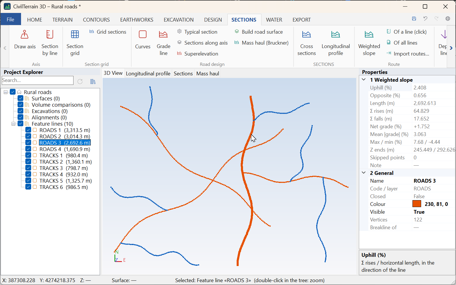
Weighted slope of all lines
SECTIONS → Route → Of all lines, or Weighted slope of all lines… in the weighted slope window and in the right-click menu of Feature lines in the tree. The table has one row for every visible 3D line of the project and stays open beside the main window. It follows the project: a new import, an edit, an undo, lines shown or hidden in the tree. If the project has no 3D lines yet, the program offers to import routes.
Columns: No., Route, Code / layer, Horizontal length (m), Σ rises ΔHv (m), Σ falls (m), Weighted slope uphill %, Opposite direction %, Net grade %, Max segment grade %, Min segment grade %, Points. The totals are shown above the table, e.g. for the sample 13_diadromes.dxf (Figure 15.11) “10 routes · 17.095 km · Σ ΔHv 469.86 m · weighted slope of all 2.749 %”: the weighted slope of all is the Σ ΔHv of all routes divided by their total length.
- Sorting: click a header (again: the other way round). Names sort with their numbers as numbers (ROADS 2 before ROADS 10).
- Click a row (or move with the arrow keys): the line is selected in the tree, its Properties open and the view zooms to it; the Zoom to button does the same.
- Details…: the full window of the route (below).
- Copy (or Ctrl+C): the selected rows (when you have selected more than one), otherwise all of them, with the headers, to paste into Excel; numbers in the Windows format.
- Excel: a Summary sheet with one row per route and a Total row, and one sheet per route in the layout of the classic sheet of section 15.6. The sheets per route are written for up to 200 routes and 250,000 vertices in all; above that the Excel has the summary only and the program says so (the table of one route: Details… → Excel).
- CSV: the summary, with
;as separator and a decimal point.
The exports follow the sorting of the table. Routes without elevations are shown in orange with 0 % and are left out of the totals, because their slope is not known: above the table it says “⚠ N without elevations (0 %): left out of the totals”, and the same note is written below the Total row of the Excel.
The Also the 3D polylines of the surfaces (breaklines) check box adds the breaklines of the visible surfaces (e.g. 3D polylines imported into a surface, section 7.2), named “surface · line”. It is ticked from the start when the project has no visible 3D lines of its own.
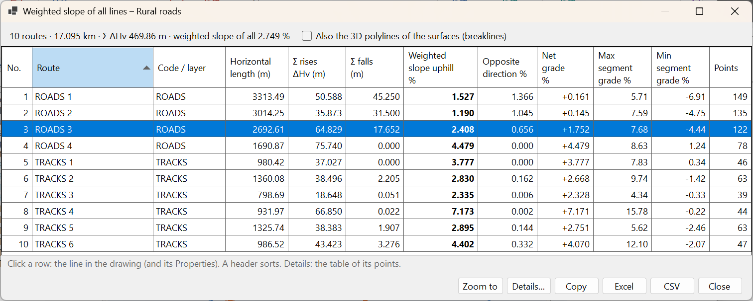
Right-click: the full window of one route
Right-click a line, in the 3D view or in the tree, and its menu opens: Zoom to (the view zooms to the line), Weighted slope… (in bold), Edit elevations…, Grade labels and Delete. Weighted slope… opens the window of section 15.6 for this line, with the table No., X, Y, Z, Station, ΔX, ΔH, Grade %, ΔHv and export to Excel or CSV. A closed line also has Platform from this line, Polygon earthworks… and Zone from this line in its menu. In the 3D view the right-click menu opens on feature lines only.
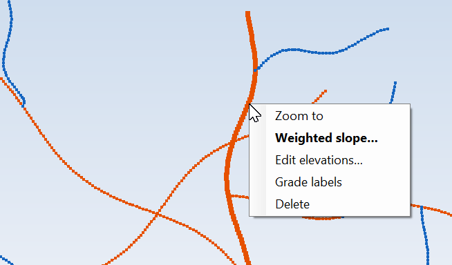
With more than 500 lines the tree groups them per code / layer (section 3.2). A project with 3D lines only is saved like any project, and the program asks whether to save it before closing.
Limits
- Every LINE entity of the DXF (a segment of two points) becomes a route of its own; the segments of an exploded drawing are not joined back into routes. Join the segments into polylines in the drawing before the import.
- Changes of name, colour and visibility in the Properties are not undone by Undo.
- Routes without elevations (2D polylines) give 0 % and do not count in the totals.
- The tree shows up to 300 lines per layer; the others are in the Item list or appear when you select them in the drawing or in the table.
16. Re-measurement with the same sections
To compare surveys from different phases (e.g. the initial survey and the survey after the works) the sections must be at exactly the same positions.
16.1 Exporting section positions
SECTIONS → Export positions saves a .ctsec file with the axis (vertices with mm precision), the widths and every section:
FORMAT;CT3D-SECTIONS;1
NAME;Axis 1
CRS;2100
START;0.000000
WIDTHS;40.000000;40.000000
VERTEX;476290.000000;4205600.000000
...
SECTION;Station;CenterX;CenterY;Azimuth(grad);LeftX;LeftY;RightX;RightY
SECTION;25.000000;476314.9940;4205601.1898;95.9604;476313.0911;4205641.1445;476316.8970;4205561.2352
It is a plain text file that opens in Excel or other software (azimuths in grads).
16.2 Re-creating sections at the same positions
- Import the new survey as a new surface and make it active.
- SECTIONS → Import positions and choose the
.ctsecfile. - In the dialog keep "Use the stored positions" checked and choose base/comparison surfaces.
- The sections are created at exactly the same positions, with the same chainages and widths.
16.3 Other section exports
| Command | Content |
|---|---|
| Section points CSV | For every section and surface: chainage, offset, X, Y, Z (real coordinates). |
| Plan DXF | Axis, section lines and chainages in real coordinates. |
| Sections PDF / DXF | Section drawings (3 per page in PDF, a grid in DXF) with areas. |
| Profile PDF | Longitudinal profile on A3 with band table. |
| Excel | Areas and cumulative volumes per section and the points of every section. |
Note: a positions file without VERTEX records (only SECTION) is also accepted; the axis is rebuilt from the section centres.
17. Road design
For rural/forest roads, accesses, platforms and small road works, CivilTerrain 3D builds the road surface from the axis, the grade line and the typical section and computes earthworks and the mass-haul diagram. The tools are in SECTIONS → Road design and in the axis right-click menu.
17.1 Horizontal alignment: arcs and clothoids
Curves: for each vertex (PI) of the axis enter a radius R and a clothoid length L (0 = none). The deflection angle (grad) and the new axis length are shown. The geometry is checked: if the tangents of two consecutive curves overlap or a clothoid is too long, a warning appears.
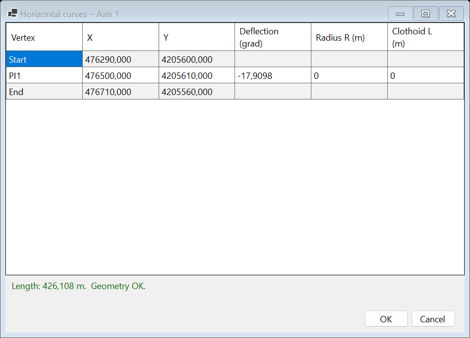
Stations, cross sections, the profile, position exports and drawings now follow the curved geometry. The key points (TS/SC/CS/ST, BC/EC) are used by the "sections at vertices" option.
17.2 Grade line (design profile)
Grade line: table of VIPs with station, elevation and vertical (parabolic) curve length. Grades are computed and the ground elevation is shown. The buttons Start/end on ground and Follow ground give a quick initial grade line.
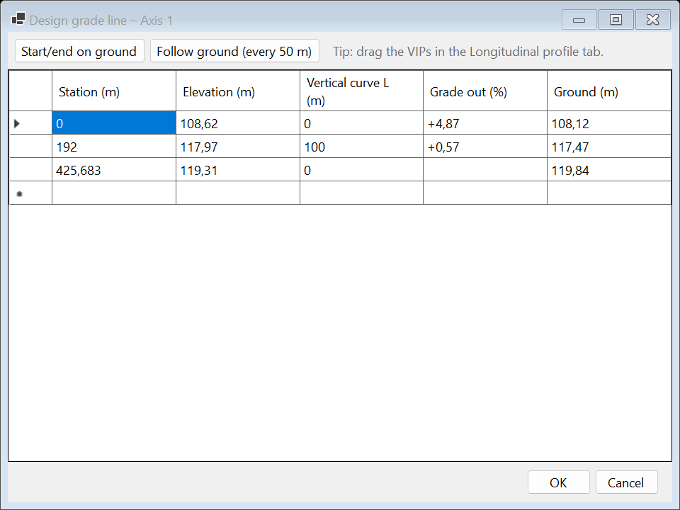
In the Longitudinal profile tab the grade line is drawn in red with grades and curve lengths. Drag the squares with the mouse to move a VIP (Shift = vertical only). The band under the profile shows design elevations and design − ground difference.
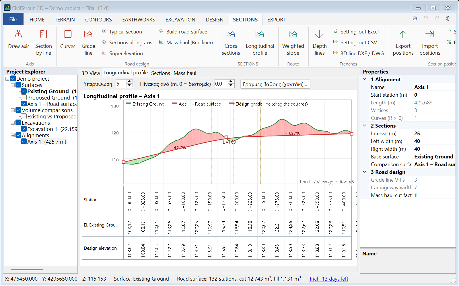
17.3 Typical section
Typical section: lane widths left/right, cross fall, shoulder width and fall, cut and fill slopes (H:1), maximum slope width and model station step. The sketch updates as you type.
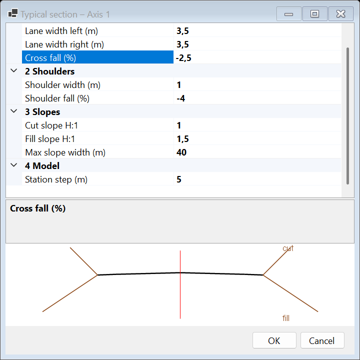
17.4 Road surface and earthworks
Build road surface: a 3D surface is created (carriageway + side slopes daylighting on the ground) together with a ground → road volume comparison. The axis is set so that the cross sections show ground and road, with cut/fill areas and volumes. After changing curves, grade line or typical section press Build road surface again to update.
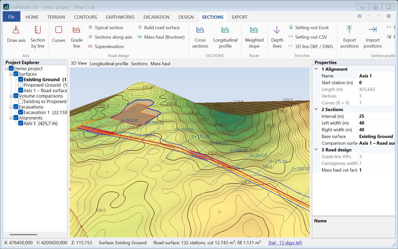
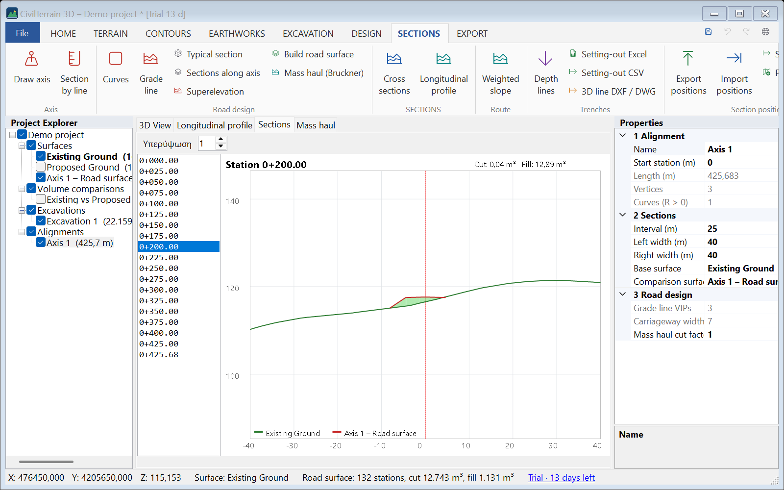
17.5 Mass-haul (Bruckner) diagram
Mass haul (Bruckner): the cumulative volume curve (cut × factor − fill) is computed from the cross sections. The cut factor expresses swell or shrinkage (e.g. 0.9). Rising parts = surplus, falling parts = deficit; crossings of the zero line are balance points. Export to Excel with Bruckner Excel.
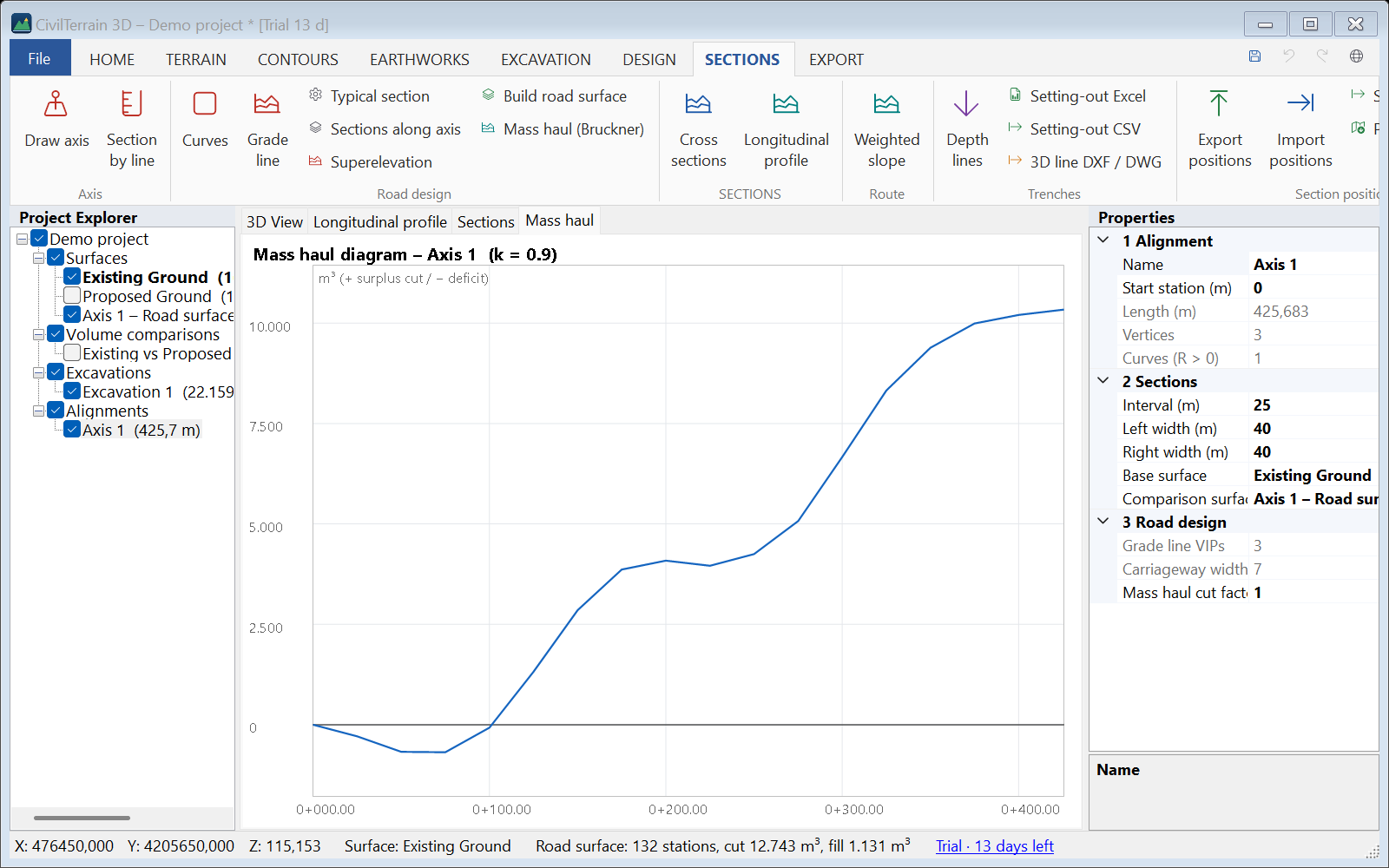
17.6 Typical sections along the axis and widenings
Sections along axis: add typical sections that apply from a station onwards (e.g. widening in a bend, different carriageway width, other slopes). The change from one to the next is linear over the transition length.
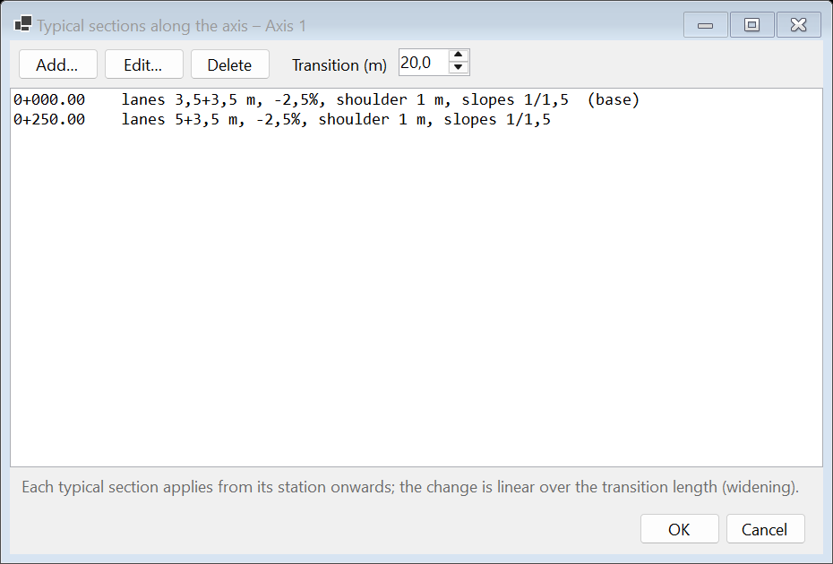
17.7 Superelevation
Superelevation: in curves the carriageway takes a single cross fall towards the inside. The rate is automatic from design speed and radius (q = V²/127R − f, limited to the maximum) or entered per curve. The run-off follows the clothoid or, without clothoid, the run-off length (2/3 on the straight, 1/3 in the arc). The superelevation diagram shows left and right cross fall along the axis.
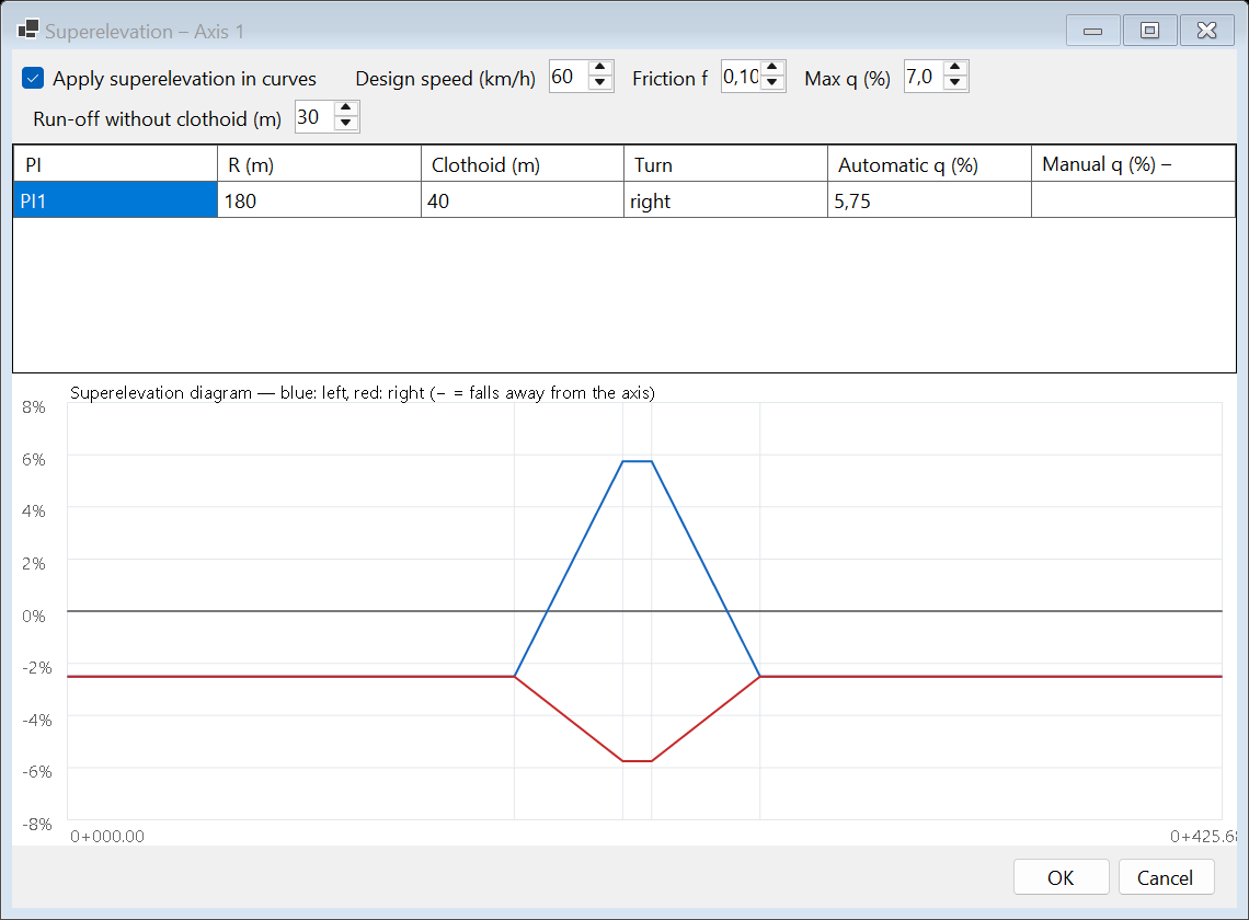
18. Dynamic labels
The labels of DESIGN → Labels are dynamic: the text is computed from the geometry, so it updates by itself when the terrain, the axis or the line changes.
| Label | Content |
|---|---|
| Spot elevation | Cross and elevation of the active surface (repeating). |
| Slope arrow | Downhill arrow with the surface slope at the point. |
| Slope between points | Surface slope between two points. |
| Axis stations | Stations at the label interval and key points (TS/ST, BC/EC). |
| Curve data | R, clothoid A and L, T, arc length and angle for each vertex. |
| Line grades | Grade and length of each segment and vertex elevations of a feature line. |
| Text | Free text. |
Label style sets text height (plan metres), decimals, elevation prefix, slope as % or 1:n and station interval. Labels appear on screen (overlapping ones are hidden until you zoom in), on PDF sheets and in the DXF/DWG drawing.
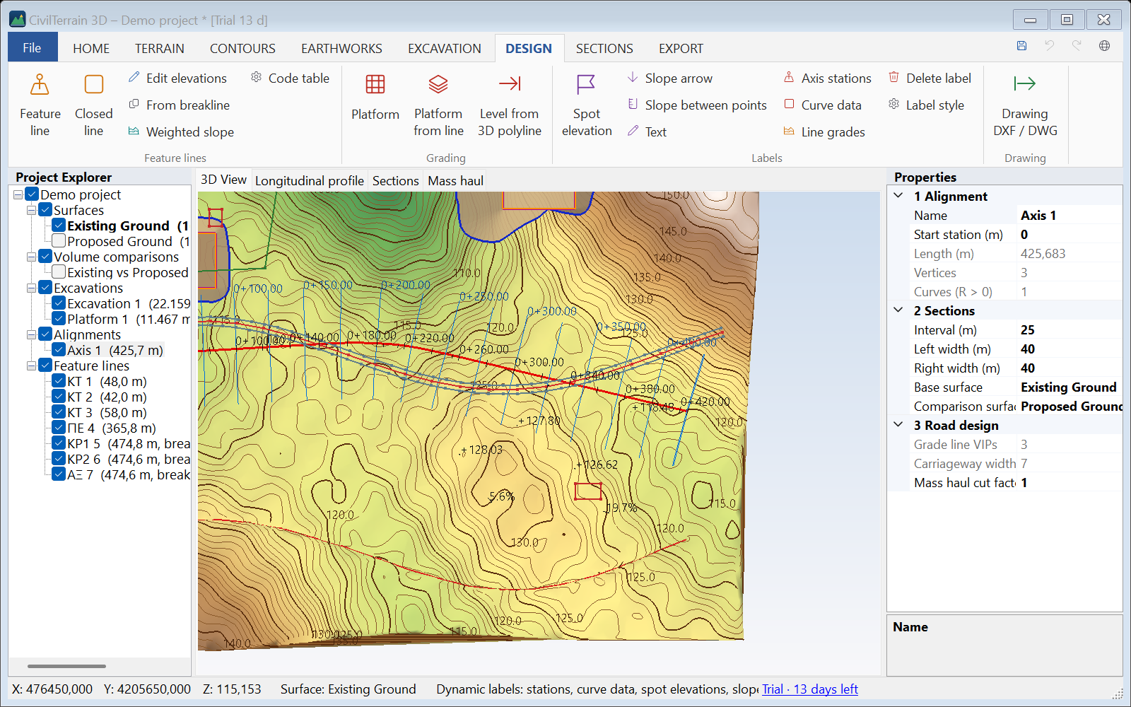
19. Technical reports
EARTHWORKS → Report PDF / Report Excel for the selected volume comparison (or EXCAVATION → Report PDF for an excavation). The PDF report contains:
- project name, date, author, coordinate system;
- the compared surfaces with points, triangles, areas and elevation range;
- the excavation data (if any);
- results: cut, fill and net volume, areas, maximum depths, cut / fill centroids and the distance between them, computation time (with topsoil: also the volumes without stripping);
- balance and haulage (loose volumes, weight, surplus / borrow, truckloads) and the waste (ΣΔΑ) table with the project factors;
- volumes per zone (all zones, continued on the next page);
- the calculation method and a page documenting it;
- a cut/fill plan with legend, scale bar, north arrow and an image of the 3D model (as currently shown on screen).
The Excel report contains sheets for results, balance – waste, surfaces, zones and, if computed, sections. The excavation report prints all parameters (cut / fill slopes, per side, platform grades, balance factor). Polygon earthworks (§12.6) and spot grids (§5.4) have their own reports.
19.1 Scaled drawing sheets
For deliverable drawings: EXPORT → Plan sheet (scale) and SECTIONS → Section sheets (scale) create PDFs on A4–A0 paper (landscape) with:
- frame, coordinate grid, north arrow and scale bar;
- a title block with title, drawing number, company/office, scale, coordinate system, date and logo;
- plan: triangles, contours with labels, axes with sections and zones (optional);
- sections: consecutive sheets with as many sections as fit, at the horizontal/vertical scale you choose (e.g. 1:200 / 1:100), with cut/fill areas.
Company and logo are stored in the project. Print the PDFs at actual size (no "Fit to page").
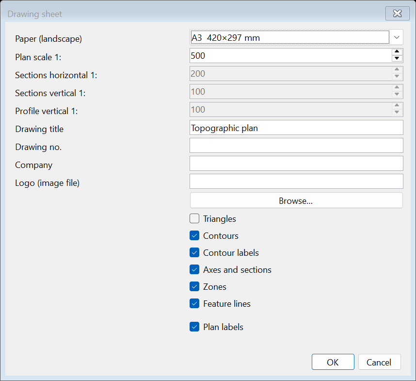
19.2 Plan-profile sheets
SECTIONS → Plan-profile sheets: the axis is split automatically into parts that fit the paper at the chosen scale. Each sheet shows the plan rotated along the part (contours, axis with stations, lines, labels, north arrow, match lines to the neighbouring sheets) above the profile of the same stations with grade line, grades, cut/fill and data band. The profile vertical scale is set separately.
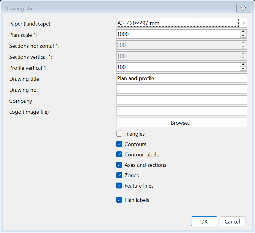
20. Exporting data
The EXPORT tab exports the active surface:
| Format | Content / notes |
|---|---|
| DXF | Triangles (3DFACE), contours, labels, breaklines, boundaries on separate layers. Compatible with all CAD (R12). |
| DWG | Every CAD export (surface, contours, sections, axis plan) can also be saved as DWG (AutoCAD 2013 format) — choose "DWG" as file type. |
| Drawing DXF / DWG | DESIGN → Drawing DXF / DWG: contours, feature lines on layers per code, axes, zones, labels, polygon earthworks (outline with design elevations, zero line, daylight) and excavation daylight / bottom — ready for AutoCAD / Civil 3D. |
| LandXML | TIN surface with breaklines and EPSG (Civil 3D and other software). |
| CSV / XYZ | TIN vertices with 0.1 mm precision. |
| Spot grid | EXPORT → Points → Spot grid: the points of a spot grid as CSV (PT,X,Y,Z,CODE), TXT (PNEZD), DXF / DWG (SG_… layers), Excel or PDF with a plan at scale (section 5.4). |
| LAS | Points as LAS 1.2 with EPSG. |
| OBJ / STL | Mesh for 3D software and printing. Writing relative to an origin is recommended (STL is always relative) to keep precision. |
| GeoTIFF | Gridded DEM with selectable cell size, georeference, NoData and .tfw / .prj files. |
| ESRI ASCII Grid | DEM as text (.asc) with selectable cell size and a .prj file — for GIS and hydraulic / hydrological software. |
| PDF plan | Plan with contours, labels and triangles. |
| Image (PNG/JPG) | The current 3D view. |
A .prj file with the project coordinate system is written next to DXF/CSV/XYZ/OBJ/STL/LAS exports.
21. Coordinate systems
| EPSG | System |
|---|---|
| 2100 | GGRS87 / Greek Grid (default) |
| 4326 | WGS 84 (geographic degrees) |
| 4258 | ETRS89 (geographic degrees) |
| 32634 / 32635 | WGS 84 / UTM 34N, 35N |
| 25834 / 25835 | ETRS89 / UTM 34N, 35N |
| 3857 | Web Mercator |
| — | Local system (no transformation) |
Transformations are applied on import (field "Source CRS" or "File coordinate system"; for DEMs the system is also read from the .prj). The Transverse Mercator projection is computed with sub-millimetre accuracy; the GGRS87 ↔ WGS84 conversion uses the official 3-parameter shift (about 1 m absolute accuracy). Elevations are not changed.
22. Shortcuts and controls
| Key / mouse | Action |
|---|---|
| Ctrl+N / O / S | New / Open / Save project |
| Ctrl+Z / Ctrl+Y | Undo / Redo |
| F5 | Rebuild the TIN of the active surface |
| Enter / double-click / right-click | Finish drawing a line or polygon |
| Backspace | Remove the last vertex while drawing |
| Esc | Cancel tool / clear selection |
| Left drag | Orbit |
| Right / middle drag, Shift+left | Pan |
| Wheel | Zoom to cursor |
| Double-click in the tree | Zoom to the item |
| Right-click (without dragging) on a feature line, in the 3D view | The menu of the line: Zoom to, Weighted slope…, Edit elevations…, Grade labels, Delete (section 15.7) |
23. Sample data
In the Samples folder of the installation (shortcut in the Start menu):
| File | Content |
|---|---|
| 00_etoimo_ergo.ct3d | Complete project with surfaces, volumes, excavation and axis |
| 01_topografiko_EGSA87.csv | 3,000 points with codes (;, decimal comma); the BL points form a ditch |
| 02_simeia.xyz | XYZ points without header |
| 03_meleti_platia.xml | Design surface (LandXML) for volume comparison |
| 04_topografiko.dxf | Points and a 3D breakline |
| 05_lidar.las | Point cloud with 200,000 points |
| 07_orthofoto.jpg (+ .jgw) | Sample orthophoto with world file for project 00 / CSV 01 |
| 08_kodikopoiisi.csv | Survey with Greek field codes (curbs ΚΡ1/ΚΡ2, axis ΑΞ, buildings ΚΤ, fence ΠΕ, trees ΔΕ) for automatic linework |
| 09_epipedo_3dpoly.dxf | Cut-and-fill level as 3D polylines (outline + ridge) for the demo project |
| 10_zones_kyvismou.dxf | Outlines of volume areas with names (texts) for the zone import and polygon earthworks |
| 11_diadromi.csv | Route points every ~20 m for the weighted slope |
| 12_dromos_lidar.las | LiDAR cloud of a road on a hillside (cut with a ditch, fill, curve, vehicles, trees, shrubs) for following a road (section 8.4); unclassified (class 1), as it comes |
| 13_diadromes.dxf | 10 routes (3D polylines) in GGRS87, 17 km in all, on the layers ROADS and TRACKS, and a 2D frame on the layer FRAME, which starts unticked in Import routes; try SECTIONS → Route → Import routes… (section 15.7) |
| 06_dem.tif | DEM on a 2 m grid |
Exercise: import 01 (with "Codes as breaklines"), then 03, create a volume comparison and a PDF report; then draw an axis and produce a profile and sections.
24. Troubleshooting
| Problem | Solution |
|---|---|
| Windows shows a warning during setup | Click "More info → Run anyway". Always download from civilshop.gr. |
| The 3D view is empty or shows "OpenGL unavailable" | Update the graphics driver. Over Remote Desktop OpenGL may not be available. |
| LAZ does not open | Put laszip64.exe in the installation tools folder or convert to LAS. |
| Points in the wrong place after import | Check the X/Y columns (or "Swap X/Y") and the "Source CRS". |
| Long "bridge" triangles at the edges | Set Max edge length or an Outer boundary. |
| Message about breaklines not inserted | Breaklines crossing boundaries or other lines inconsistently; check the data. |
| "Could not contact the license server" | Check Internet/firewall. The program keeps working for 7 days offline. |
| "This TIFF is a picture, not elevations" | The file is a coloured image (e.g. an elevation map). Ask for the DEM with elevation values (e.g. Float32 or Int16) or load the image as an orthophoto. |
| The DEM appears far from the project | Check the "File coordinate system" in the DEM import dialog (e.g. WGS 84 for SRTM and Copernicus, GGRS87 for Hellenic Cadastre DEMs). |
| Slow with very large files | Use grid thinning when importing LAS, or DEM thinning. |
| Trucks and machines in a drone survey count in the volumes | TERRAIN → Remove objects (section 10.4): automatic detection, check the list, Apply. For debris or a pile inside an excavation: Replace terrain (section 10.5). The ground filter does not run on a triangle mesh (DEM / DSM, LandXML, OBJ / PLY). |
| The spot grid is not created (“Too many points (more than 250,000)…”) or its DWG is not written | A spot grid takes up to 250,000 points: increase the spacing or make the perimeter smaller. A DWG is written for up to 50,000 points; save it as DXF (the same layers) or CSV. |
| How do I get the weighted slope of many routes without a ground surface? | SECTIONS → Route → Import routes…: the 3D polylines of the DXF / DWG become 3D lines without a surface. Click a line: its weighted slope is in the Properties; all of them together are in the Weighted slope of all lines table, with Excel / CSV (section 15.7). |
The error log is in %APPDATA%\CivilTerrain3D\error.log; send it with a description of the problem to Info@civilshop.gr.
25. Technical notes and accuracy
- Triangulation: Delaunay (sweep-hull, O(n log n)) with constrained edges for breaklines and boundaries; crossing breaklines are split automatically.
- Coordinate precision: all calculations are in double precision in a local reference frame; GGRS87 coordinates are kept without rounding.
- Volumes: exact overlay of the two TINs (triangle intersection) and integration of the linear elevation difference on every polygon, with an exact split at the zero-difference line. No grid approximation is used.
- Contours: computed from the TIN edges as topologically continuous lines.
- Excavation: slopes are defined as the union of per-side wedges; the daylight line is found numerically (marching and bisection) on the real TIN.
- Verification: the software is tested automatically against examples with known results (pyramid, inclined planes, frustum, Steiner formula for pits, etc.).
- Performance: TIN of 300,000 points in about 1 second; volume comparison of 300,000 × 100,000 triangles in about 2 seconds (typical laptop).
- Remove objects / replace terrain: the new ground is computed on a grid inside the outlines, with the elevations held on a strip about 1 m wide around them. Smooth surface: the Laplace equation (a membrane) solved by conjugate gradients; plane: least squares; lowest level: about the 5th percentile of the strip; both for each outline (together for outlines that touch or overlap). Up to 500,000 nodes per computation; on larger outlines the spacing grows by itself. The removed / added volumes are the cut and fill between the TIN before and after, measured on the triangles that changed (the same as a volume comparison of the two surfaces).
- Automatic object detection: the surface is turned into a 0.25 – 0.5 m grid; a morphological opening with a window as large as the largest machine gives the ground, and every group of cells more than 0.80 m above it is checked for size, plan, steep sides, a flat top and lower, even ground around. The shape measures are taken from areas within contours, not from single cells, so noise does not make a pile look like a machine.
- Spot grid: the elevation of every point is interpolated linearly on the TIN triangle that holds it; up to 250,000 points per grid. A point of the perimeter within 2% of the spacing of a grid node (at most 5 cm, at least 2.5 mm) is that node.